P. 4 ~ Continued - LOUISIANA HAYNESVILLE SHALE—1: Characteristics, production potential of Haynesville shale wells described
Displaying 4/6
View Article as Single page
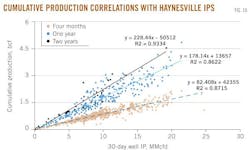
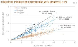
IP-cumulative production
In Fig. 10, cumulative gas production after 4 months, 1 year, and 2 years is correlated with well IP rate for Haynesville wells. As the time period increases, the slope of the relationship increases because cumulative production increases.
Recovery statistics
Estimated ultimate recovery
Estimated ultimate recovery is a function of initial production, decline rate, economic limit, gas price, formation characteristics, completion strategy, and related factors.
We cannot control for most of these factors, and because public data on formation and completion characteristics are limited, constraints exist in our ability to incorporate these factors in analysis.
The number and interaction of these and other parameters create more variables than can currently be discriminated.
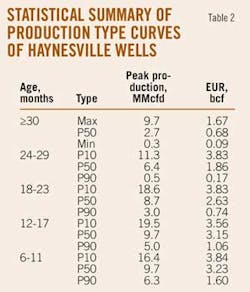
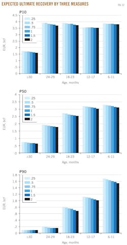
A summary of computed EURs is shown in Table 2 by vintage and average well type. EUR is estimated based on exponential and hyperbolic decline curve models. Production is assumed to terminate at an economic limit (EL) of 90 Mcfd.
P10 reserves dominate each vintage category and are bound above by 4 bcf/well. P50 wells generally range from 1.9 to 3.2 bcf/well. P90 wells range from 0.2 to 1.6 bcf/well. The EUR values appear low relative to company estimates and industry expectations.
Sensitivity analysis
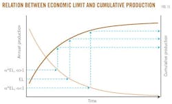
The economic limit for North Louisiana gas fields was previously shown to average 41 Mcfd,14 a value about half of the assumed cutoff level. If the actual EL is smaller than the baseline assumption, production will reach its commercial threshold later and produce more on a cumulative basis, and vice versa, if the EL increases cumulative production will decline (Fig. 11).
The results of sensitivity analysis are shown in Fig. 12 per production class by vintage and economic limit multiplier. EUR changes about 10% for a tenfold change in EL, so for practical purposes, threshold-level induced changes in EUR are considered negligible.
IP-EUR correlation
Initial production per vintage class profile is correlated against EUR in Fig. 13 based on the data in Table 2. An approximate linear relationship exists between IP and EUR:
EUR (bcf) = 0.35 + 0.00021 IP (MMcfd).
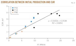
We observe:
• Low IP rates associated with P90 curves correspond to EURs below 2 bcf.
• High IP rates associated with P10 curves correspond to EURs between 2 and 4 bcf.
• P50 profiles correspond to EURs between 1 and 3 bcf.
The effectiveness of the fracture system, not the IP rate, is the determining factor in long-term production and EUR. IP cannot evaluate fracture effectiveness, and so the derived correlation is a modeling artifact rather than a reflection of the physics of the production reservoir. Thus, the validity of the generalized correspondence is suspect and the relation is only applied to estimate the EUR distribution.
EUR distribution
Using the relationship between IP and EUR, it is straightforward to estimate the EUR distribution for the inventory of single-well LUWs (Fig. 14).
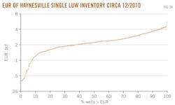
The December 2010 inventory of single-well LUWs range from less than 0.5 bcf/well to over 4 bcf/well. About 40% of Haynesville wells are expected to yield EURs between 2 and 3 bcf/well, 30% less than 2 bcf/well, and 30% greater than 3 bcf/well. The current inventory of single-well LUWs is estimated to have total reserves of 1,837 bcf.
Displaying 4/6
View Article as Single page