P. 3 ~ Continiued - LOUISIANA HAYNESVILLE SHALE—1: Characteristics, production potential of Haynesville shale wells described

Displaying 3/6
View Article as Single page
IP rates in unconventional plays tend to reflect how much rock has been exposed by a given completion. As the length of the lateral and total number of stages increases, IP is expected to increase. In previous studies, high IP wells were shown to be correlated in structurally thin areas and high free-gas porosity regions.2 3 Structural thinness enables effective stimulation of the entire interval, and low smectite/high calcite areas enable the interval to be stimulated easier because calcite is stiff and hard and high calcite content reduces the risk of proppant embedment.
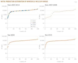
Fig. 8 presents IP distribution by well vintage. IP rates vary widely. Wells brought on line within the last 2 years peak higher than older wells, which is likely the result of better identification on core production areas and better experience with fracture technology. In 2009-10, half of all new wells had an IP greater than 10 MMcfd and 80% of all wells had peak production of 4 to 16 MMcfd.
Production statistics
Type curves
We group wellbores by age and compute average profiles initialized from first production using single-well LUWs with production history through December 2010.
The data set consists of 683 wells. We do not consider multiple-well LUW profiles because of the additional processing required to normalize well count.
Averaging reduces extreme characteristics, smoothes out volatility, and normalizes production for departures in operating practices. Average curves provide a general representation of well production potential and is a useful means to assess productivity. The average profile is referred to as the P50 curve.
P10, P50, P90 profiles
The average monthly production profiles for Haynesville wells by vintage are depicted in Fig. 9.
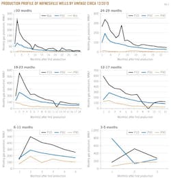
Wells are categorized by age into six vintage classes: ≤5, 6-11, 12-17, 18-23, 24-29, and ≥30 months. In addition to the average production profiles, we also present P10 and P90 curves. P10 represents the production profile of the well where 10% of the category wells exceed its cumulative production at the beginning of the time period; P90 represents the well where 90% of the category wells exceed its cumulative production at the beginning of the time period.
Unlike P50 which represents the average profile of the sample set, P10 and P90 curves represent a specific well ranked and selected according to cumulative production. P10 and P90 represent individual wells and exhibit greater volatility relative to P50 since they are not average profiles.
Decline curves
Steep decline is a common characteristic of shale plays because of formation and completion characteristics,7-9 and Haynesville wells are no exception.
Early production is typically dominated by the permeability of the fracture system, fracture spacing, and effective lateral length. Over time, other properties begin to influence decline and the rate of change of decline begins to slow.
For Haynesville wells, the average completion declines rapidly and produces 80% of its expected recovery during the first 2 years of production.
Production histories from Haynesville wells are not well established, and so estimation of decline curves and reserves is subject to great uncertainty.
Each profile in Fig. 9 was modeled using decline curves that are an approximation of reservoir dynamics. Precise fits does not imply better predictive performance.
Failure to recognize extended transient regimes will cause conventional models and recovery volume predictions to be pessimistic.10-13 If exponential decline is the initial best-fit model for a reservoir that eventually exhibits a hyperbolic decline trend, reserves estimates will be underestimated. Conversely, initial best-fit hyperbolic declines for reservoirs that later exhibit exponential decline will overstate reserves.
Displaying 3/6
View Article as Single page