LOUISIANA HAYNESVILLE SHALE—1: Characteristics, production potential of Haynesville shale wells described
Mark J. Kaiser
Yunke Yu
Louisiana State University
Baton Rouge
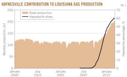
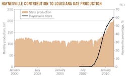
The contribution of the Haynesville shale to Louisiana's gas production has been phenomenal: After 3 years, almost 60% of the state's gas output is now sourced from the Haynesville (Fig. 1).
The Haynesville is the deepest, hottest, and highest pressured shale among the big four plays (the others being Barnett, Fayetteville, and Marcellus) and also the most expensive, with drilling and completion cost at $7-10 million/well. The potential rewards are great, however, with initial production averaging 10 MMcfd and expected recoveries of 2-4 bcf/well.
The purpose of this article is to describe the productivity characteristics of Haynesville wells, project future production from the inventory of active wells, and assess production potential based on hypothetical drilling scenarios. In Parts 2 and 3 of this series we will describe the operating envelope under which Haynesville wells are expected to be economic and characterize the profit space.
In this article, we offer statistical analysis of wells drilled to date and construct type profiles to characterize the play. We also compute the distribution of expected ultimate recovery per foot of perforation length.
We estimate that the current inventory of producing wells will extract 3 tcf over their life cycle, and within the next 3 years, cumulative build-out in the region will range between 3 and 9 tcf. To maintain current gas production levels in the state near-term, we estimate that about 550 shale gas wells/year will need to be completed over the next 3 years.
Geology and reservoir characteristics
The Haynesville shale is one of several unconventional gas plays that have been discovered in the US in recent years and promise to dramatically change the course of future domestic energy development.1
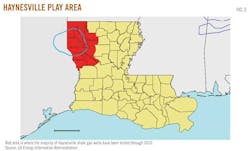
The Haynesville shale play covers 9,000 sq miles across East Texas and Northwest Louisiana (Fig. 2). The Haynesville was laid down during the Upper Jurassic and is overlain by the Bossier shale followed by the Cotton Valley sandstone. It is underlain by the Cotton Valley limestone in Texas and the Smackover limestone in Louisiana.2
Wells targeting the Haynesville shale are typically drilled to vertical depths of 11,000-12,500 ft and have horizontal laterals of 4,000-5,500 ft. The Haynesville is unique because of its abnormally high pressures of 0.72-0.90 psi/ft and temperatures greater than 300° F. The high reservoir pressure was created when the organic material in the shale broke down into gas but remained trapped in the source rock because of impenetrable surrounding rock layers.
Sedimentation from ancestral rivers thickened the Haynesville along the Arkansas-Louisiana line to 400 ft. To the south, the Haynesville interval thins to 180 ft through Bossier, Red River, and DeSoto parishes in Louisiana and Shelby County, Texas.3 Some sections are highly pressurized with faults, clay deposits, and other factors contributing to drilling complexity and risk. The highest-producing wells occur in an area where the interval is thin with high calcite and low clay content.4 5
Most regions are thermally mature and contain only dry gas. Through December 2010, 1.56 tcf had been extracted from the play with 20,500 bbl of condensate. Estimates of technically recoverable resources range between 73 tcf and 289 tcf, making the Haynesville one of the largest shale plays in the US.
Well statistics
Data source
The Louisiana Department of Natural Resources maintains drilling data in the SONRIS system and identifies separately Haynesville wells.6
Data on drilling activity include spud date, location, field name, lease type, operator, vertical depth, measured depth, perforation interval, and other physical features of the well construction (e.g., tubing size, casing size) and test data (e.g., production, pressure, choke size).
Additional information on drilling and completion activities is based on scout sheets. Production activity is reported monthly in terms of lease unit well (LUW) administrative codes. Single-well LUWs involve one well product streams; multiple-well LUWs report aggregate production based on more than one well.
Production growth
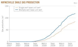
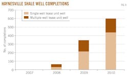
Haynesville shale gas production by single-well and multiple-well LUW is shown in Fig. 3. The majority of production arises from single-well LUWs. There have been 1,052 shale gas completions through December 2010 with 683 single-well LUWs and 234 multiple-well LUWs (Fig. 4).
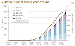
The growth in gas production is a direct result of the large number of new wells that have been brought into production in DeSoto, Caddo, and Red River parishes (Fig. 5). Well completions track production trends closely because the play is still in the early stages of development and marginal inventories are small. As production matures and wells age, the correlation between the number of active wells and production will begin to diverge.
Well configuration
To date, 75% of Haynesville wells have been drilled to 11,000 to 12,500 ft TVD and 20% of wells have been drilled between 12,500 to 14,000 ft TVD (Fig. 6). The measured depth of most wells ranges between 16,000 to 18,000 ft, indicating the high deviation and horizontal displacement of well trajectories.
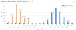
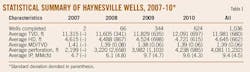
Average vertical depth of well construction has increased to 12,091 ft in 2010 from 11,605 ft in 2008 as the core areas of the play have become established (Table 1).
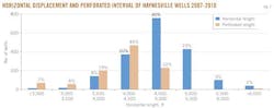
Over 80% of Haynesville wells have a horizontal displacement between 4,000 ft and 5,500 ft and a perforated interval of 3,500 ft and 5,000 ft (Fig. 7). Variation in horizontal displacement and perforated interval is large and reflects differences in completion strategies among operators. Perforation length is the most variable of all well parameters and is an important element in design since it is a key factor in the tradeoff between revenue and cost.
Initial production
Initial production (IP) is an indicator of deliverability and is a standard measure of well quality.
We normalize and report on a daily basis IP rates by well vintage. The average IP for all wells that started producing in 2008 was 6.1 MMcfd; in 2009-10, average IP rates increased to 9.7 MMcfd (Table 1).
Many factors contribute to well productivity, including the depth, thickness, and lateral extent of the shale; organic richness; thermal maturation; permeability and pore pressure; stimulation success; and completion strategy (e.g., perforated interval, number of frac stages, and proppant volume).
IP rates in unconventional plays tend to reflect how much rock has been exposed by a given completion. As the length of the lateral and total number of stages increases, IP is expected to increase. In previous studies, high IP wells were shown to be correlated in structurally thin areas and high free-gas porosity regions.2 3 Structural thinness enables effective stimulation of the entire interval, and low smectite/high calcite areas enable the interval to be stimulated easier because calcite is stiff and hard and high calcite content reduces the risk of proppant embedment.
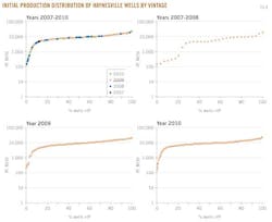
Fig. 8 presents IP distribution by well vintage. IP rates vary widely. Wells brought on line within the last 2 years peak higher than older wells, which is likely the result of better identification on core production areas and better experience with fracture technology. In 2009-10, half of all new wells had an IP greater than 10 MMcfd and 80% of all wells had peak production of 4 to 16 MMcfd.
Production statistics
Type curves
We group wellbores by age and compute average profiles initialized from first production using single-well LUWs with production history through December 2010.
The data set consists of 683 wells. We do not consider multiple-well LUW profiles because of the additional processing required to normalize well count.
Averaging reduces extreme characteristics, smoothes out volatility, and normalizes production for departures in operating practices. Average curves provide a general representation of well production potential and is a useful means to assess productivity. The average profile is referred to as the P50 curve.
P10, P50, P90 profiles
The average monthly production profiles for Haynesville wells by vintage are depicted in Fig. 9.
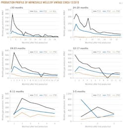
Wells are categorized by age into six vintage classes: ≤5, 6-11, 12-17, 18-23, 24-29, and ≥30 months. In addition to the average production profiles, we also present P10 and P90 curves. P10 represents the production profile of the well where 10% of the category wells exceed its cumulative production at the beginning of the time period; P90 represents the well where 90% of the category wells exceed its cumulative production at the beginning of the time period.
Unlike P50 which represents the average profile of the sample set, P10 and P90 curves represent a specific well ranked and selected according to cumulative production. P10 and P90 represent individual wells and exhibit greater volatility relative to P50 since they are not average profiles.
Decline curves
Steep decline is a common characteristic of shale plays because of formation and completion characteristics,7-9 and Haynesville wells are no exception.
Early production is typically dominated by the permeability of the fracture system, fracture spacing, and effective lateral length. Over time, other properties begin to influence decline and the rate of change of decline begins to slow.
For Haynesville wells, the average completion declines rapidly and produces 80% of its expected recovery during the first 2 years of production.
Production histories from Haynesville wells are not well established, and so estimation of decline curves and reserves is subject to great uncertainty.
Each profile in Fig. 9 was modeled using decline curves that are an approximation of reservoir dynamics. Precise fits does not imply better predictive performance.
Failure to recognize extended transient regimes will cause conventional models and recovery volume predictions to be pessimistic.10-13 If exponential decline is the initial best-fit model for a reservoir that eventually exhibits a hyperbolic decline trend, reserves estimates will be underestimated. Conversely, initial best-fit hyperbolic declines for reservoirs that later exhibit exponential decline will overstate reserves.
IP-cumulative production
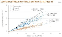
In Fig. 10, cumulative gas production after 4 months, 1 year, and 2 years is correlated with well IP rate for Haynesville wells. As the time period increases, the slope of the relationship increases because cumulative production increases.
Recovery statistics
Estimated ultimate recovery
Estimated ultimate recovery is a function of initial production, decline rate, economic limit, gas price, formation characteristics, completion strategy, and related factors.
We cannot control for most of these factors, and because public data on formation and completion characteristics are limited, constraints exist in our ability to incorporate these factors in analysis.
The number and interaction of these and other parameters create more variables than can currently be discriminated.
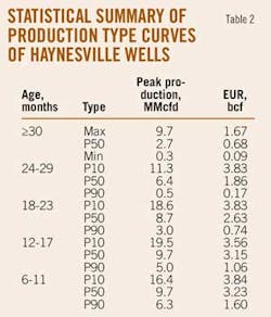
A summary of computed EURs is shown in Table 2 by vintage and average well type. EUR is estimated based on exponential and hyperbolic decline curve models. Production is assumed to terminate at an economic limit (EL) of 90 Mcfd.
P10 reserves dominate each vintage category and are bound above by 4 bcf/well. P50 wells generally range from 1.9 to 3.2 bcf/well. P90 wells range from 0.2 to 1.6 bcf/well. The EUR values appear low relative to company estimates and industry expectations.
Sensitivity analysis
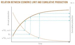
The economic limit for North Louisiana gas fields was previously shown to average 41 Mcfd,14 a value about half of the assumed cutoff level. If the actual EL is smaller than the baseline assumption, production will reach its commercial threshold later and produce more on a cumulative basis, and vice versa, if the EL increases cumulative production will decline (Fig. 11).
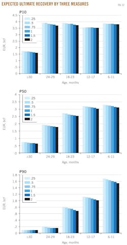
The results of sensitivity analysis are shown in Fig. 12 per production class by vintage and economic limit multiplier. EUR changes about 10% for a tenfold change in EL, so for practical purposes, threshold-level induced changes in EUR are considered negligible.
IP-EUR correlation
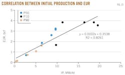
Initial production per vintage class profile is correlated against EUR in Fig. 13 based on the data in Table 2. An approximate linear relationship exists between IP and EUR:
EUR (bcf) = 0.35 + 0.00021 IP (MMcfd).
We observe:
• Low IP rates associated with P90 curves correspond to EURs below 2 bcf.
• High IP rates associated with P10 curves correspond to EURs between 2 and 4 bcf.
• P50 profiles correspond to EURs between 1 and 3 bcf.
The effectiveness of the fracture system, not the IP rate, is the determining factor in long-term production and EUR. IP cannot evaluate fracture effectiveness, and so the derived correlation is a modeling artifact rather than a reflection of the physics of the production reservoir. Thus, the validity of the generalized correspondence is suspect and the relation is only applied to estimate the EUR distribution.
EUR distribution
Using the relationship between IP and EUR, it is straightforward to estimate the EUR distribution for the inventory of single-well LUWs (Fig. 14).
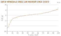
The December 2010 inventory of single-well LUWs range from less than 0.5 bcf/well to over 4 bcf/well. About 40% of Haynesville wells are expected to yield EURs between 2 and 3 bcf/well, 30% less than 2 bcf/well, and 30% greater than 3 bcf/well. The current inventory of single-well LUWs is estimated to have total reserves of 1,837 bcf.
EUR per foot distribution
Lateral length affects production rates and recovery. It might be expected, for example, that a 4,000 ft lateral with 12 stages of fracturing will produce about twice as much as a 2,000 ft lateral with 6 stages, for all other things equal.
We apply the expression EUR/FT to express the ultimate recovery per foot of lateral length. EUR units are in thousand cubic feet. Lateral length is calculated as the distance between the most distal and proximal perforations of the wellbore.
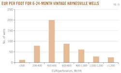
The distribution of EUR/FT is depicted in Fig. 15. The metric provides a quick assessment of production potential and economics and has been used to book proved undeveloped reserves.15
Production forecast
Current inventory
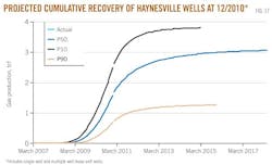
P10, P50, and P90 production profiles are used with a count of the total number of wells completed to project future production from the current inventory. The results are shown in Figs. 16 and 17.
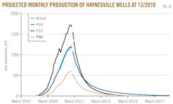
With no additional investment and no new drilling, annual production will decline and the cumulative curves will inflect and begin to converge to their expected cumulative production levels. The expected cumulative production based on P50 wells is 3 tcf. Under the P10 scenario, cumulative production may achieve 3.8 tcf; for the P90 scenario, production is expected to reach 1.3 tcf.
The message of Fig. 16 is clear. Unless new wells are continually brought on stream, Haynesville production will drop off immediately and rapidly.
Operators manage drilling programs based on capital budget constraints, current and expected future gas prices, and the need to hold acreage. The ability to bring on production quickly and reliably in a factory-like mode is an advantage in shale plays, but low price environments and high drilling cost represent constraining factors in profitability.
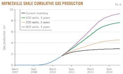
Drilling scenarios
We illustrate the expected impact of drilling activity on shale gas production using three drilling scenarios ranging from 200 wells/year to 600 wells/year to 800 wells/year for the next 3 years.
We assume future wells will follow P50 production paths described by wells 6-24 months old, a constant level of drilling activity for each of the next 3 years, and no pipeline infrastructure constraints. Prices are assumed to be maintained at a level where there is no significant production curtailment, believed to range between $4 and $5/Mcf.
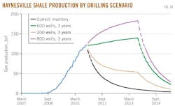
Under these assumptions, three production forecasts depict a cumulative build out ranging between 3 and 9 tcf by September 2015 (Figs. 18 and 19).
References
1. "Modern Shale Gas Development in the United States: A Primer," US Department of Energy, 2009 (http://www.netl.doe.gov/technologies/oil-gas/publications/EPreports/Shale_Gas_ Primer_2009.pdf).
2. Thompson, J.W., Fan., L., Grant, D., Martin, R.B., Kanneganti, K.T., and Lindsay, G.J., "An overview of horizontal well completions in the Haynesville shale," CSUG/SPE 136875, Canadian Unconventional Resources & International Petroleum Conference in Calgary, Alta., Canada, Oct. 19-21, 2010.
3. Pope, C., Peters, B., Benton, T., and Palisch, T., "Haynesville shale—one operator's approach to well completions in this evolving play," SPE 125079, SPE Annual Technical Conference and Exhibition, New Orleans, Oct. 4-7, 2009.
4. Kulkarni, P., "Mergers and acquisitions support sustained Haynesville drilling," World Oil, June 2010, pp. D67-D74.
5. Wang, P.F., and Hammes, U., "Effects of petrophysical factors on Haynesville fluid flow and production," World Oil, June 2010, pp. D63-D66.
6. Well Information, LDNR Office of Conservation (http://sonlite.dnr.state.la.us/sundown/cart_prod/cart_con_wellinfo1).
7. Baihly, J., Atlman, R., Malpani, R., and Luo, F., "Shale gas production decline trend comparison over time and basins," SPE 135555, SPE Annual Technical Conference and Exhibition, Florence, Italy, Sept. 19-22, 2010.
8. Anderson, D.M., Nobakht, M., Moghadam, S., and Mattar, L., "Analysis of production data from fractured shale gas wells," SPE 131787, SPE Unconventional Gas Conference, Pittsburgh, Feb. 23-25, 2010.
9. Sutton, R.P., and Cox, S.A., "Shale gas plays: a performance perspective," SPE 138447, SPE Tight Gas Completions Conference , San Antonio, Nov. 2-3, 2010.
10. Anderson, D.M., Stotts, G.W.J., Mattar, L., Ilk, D., and Blasingame, T.A., "Production Data Analysis—Challenges, Pitfalls, Diagnostics," SPE 102048, SPE Annual Technical Conference and Exhibition, San Antonio, Sept. 24-27, 2006.
11. Ilk, D., Jenkins, C.D., and Blasingame, T.A., "Production Analysis in Unconventional Reservoirs—Diagnostics, Challenges, and Methodologies," SPE 144376, North American Unconventional Gas Conference and Exhibition, The Woodlands, Tex., June 14-16, 2011.
12. Strickland, E., Purvis, D., and Blasingame, T., "Practical Aspects of Reserve Determinations for Shale Gas," SPE 144357, North American Unconventional Gas Conference and Exhibition, The Woodlands, Tex., June 14-16, 2011.
13. Lee, W.J., and Sidle, R.E., "Gas Reserves Estimation in Resource Plays," SPE 130101, SPE Unconventional Gas Conference, Pittsburgh, Feb. 23-25, 2010.
14. Kaiser, M.J., "Economic limit of field production in Louisiana," Energy—The International Journal, Vol. 35, No. 8, pp. 3,399-3,416.
15. Dobson, M.L., Lupardus, P.D., Divine, T.W., and McLane, M.A., "A Practical Solution for Booking PUD Reserves in a Resource Play Using Probabilistic Methods," SPE 144383, North American Unconventional Gas Conference and Exhibition, The Woodlands, Tex., June 14-16, 2011.
The authors


More Oil & Gas Journal Current Issue Articles
More Oil & Gas Journal Archives Issue Articles
View Oil and Gas Articles on PennEnergy.com