Alaska's oil and gas production tax severely limits upside profit potential

Roger Marks,Consulting Petroleum Economist, Anchorage, Alaska
Alaska's oil (and gas) production (or severance) tax, called "ACES" (Alaska's Clear and Equitable Share), was enacted in 2007 (effective July 1 of that year). The tax has a base tax rate of 25% on the net value of oil, the value after all exploration, development, production, operating, and transportation costs are deducted.
There is also a progressivity element (calculated monthly) that is added to the base tax rate. Progressivity is the practice of increasing the tax rate as income increases. In ACES the tax rate rises as per barrel net value increases, and is applied to the total net value. Progressivity starts as per barrel net value rises above $30/bbl. (At current [summer 2010] costs [about $25/bbl] this is equal to about a $55/bbl US West Coast Alaska North Slope [ANS] crude oil market price.) Progressivity rises at a rate of 0.4% for every per barrel dollar of net value above $30. Above $92.50/bbl in net value the progressivity rate increase drops to 0.1%/dollar of net value.
The formula for the total tax rate, including the base rate and progressivity is:
0.25 + ((Net per barrel value - $30) X .004)
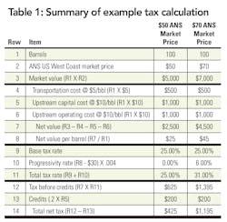
ACES also contains a 20% tax credit for capital costs, with potential greater credits for exploration depending on location. For example, let's assume the following:
- 100 barrels sold on the US West Coast
- ANS West Coast price of $50
- Transportation cost (pipeline and marine shipping) of $5
- Upstream (exploration, development, production) costs of $20: $10 capital and $10 operating
- No royalties (for simplification)
The net value of the oil would be:
100 X ($50 — $5 — $20) = $2,500
The per barrel net value would be:
$2,500 / 100 = $25/bbl
Since this is less than $30/bbl there is no progressivity and only the base tax rate would apply. Thus the tax before credits would be:
.25 X $2,500 = $625
The capital credits would be:
.20 X $10 = $200
The tax net of credits would be:
$625 - $200 = $425
Now let's say the price of oil goes up to $70.
The net value of the oil would be:
100 X ($70 — $5 — $20) = $4,500
The per barrel net value would be:
$4,500 / 100 = $45/bbl
Since this is more than $30/bbl there would be a progressivity surcharge. The surcharge would be:
($45 — $30) X .004 = .06
Thus 6% would be added to the base tax rate of 25% for a total tax rate of 31%. Thus the tax before credits would be:
.31 X $4,500 = $1,395
The capital credits would be:
.20 X $10 = $200
The tax net of credits would be:
$1,395 - $200 = $1,195
Table 1 summarizes this example. Notice that the progressivity surcharge applies to the entire net value. Also notice that as the price increased 40% (from $50 to $70), the tax increased 181% (from $425 to $1,195).
Bracketed vs non-bracketed progressivity
Progressivity is not unique among oil and gas jurisdictions, or even among non-oil taxes. In fact, the US personal income tax code contains progressivity. The tax rate for a single taxpayer in 2009 is shown in Table 2:
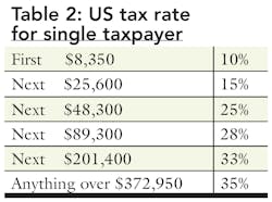
No matter how much money you make, the first $8,350 of taxable income pays at a 10% rate. The next $25,600 pays at a 15% rate, and so forth, until if you have more than $372,950 in taxable income, only anything above that amount pays at the highest rate.
Nearly all progressive tax systems, domestic and international, oil or non-oil, operate like this. There are incremental income brackets and only the amounts in the higher brackets pay the higher rates. The tax rates for the income made in the lower brackets never change.
With ACES, however, there are no brackets; as the price goes up, the new higher tax rate applies to the total net value, so the tax increases for every single dollar of net value. So if there is $1/bbl in net value, the tax rate would be just the base rate of 25%. And if there is $30/bbl in net value, the tax rate would be just the base rate of 25%. But if net value goes to $31/bbl, progressivity kicks in, and the higher rate applies not only to the 31st dollar, but to all the previous first 30 dollars as well.
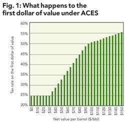
Figure 1 shows what happens to the taxation on the first dollar of value as net value per barrel goes up. It is difficult to find any other progressivity structure anywhere that operates similarly. (See International Comparison section.)
Marginal tax rates
The result is that as prices go up, and the tax rate goes up, the higher tax rate applies to every previous dollar of value, not just the last one. Whereas Figure 1 illustrated what happens to the first dollar, we can also examine what happens simultaneously to all the previous dollars of value together as prices go up.
This is shown through the marginal tax rate; when the price of oil goes up a dollar, the marginal tax rate is how much of that dollar goes to government. Under the ACES structure, when price goes up a dollar, the increased taxes from all the previous dollars get rolled into the last one, and the marginal tax rate is ever increasing.
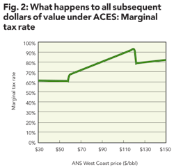
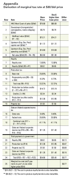
This is shown on in Figure 2. The graph shows the marginal tax rate at various ANS market prices. (Note that Figure 1 was based on net values [market prices less costs.]) These were derived from publicly available cost data from the Alaska Department of Revenue, amounting to about $25 per barrel. (Estimated capital costs are $10.20/bbl, operating costs are $9.30/bbl, and transportation costs are $5.79/bbl.) The payments to government include royalties, property tax, and state and federal corporate income taxes, as well as the production tax (which is the biggest piece: see Appendix).
At the current (summer 2010) oil market price of about $80 per barrel the marginal tax rate is 77%. This means as price goes from $79 per barrel to $80 per barrel the government would get 77 cents out of that dollar increase, 47 cents of which is the production tax. (The other 30 cents are 13 cents for the royalty and 17 cents for the income tax. (See Appendix for depiction of the detailed derivation of the marginal tax rate.)
(Because the rate of increase drops from 0.4% to 0.1% when net value exceeds $92.50 [a market price of about $120], the marginal tax rate declines to about 80% at that point and then starts increasing again, albeit at a slower rate.)
The rate increases are entirely attributable to the production tax. The property tax is based on property value so it is a flat nominal amount regardless of price (about $1.50 per barrel). The royalty is a fixed percentage of the wellhead value (market price less transportation costs). The state and federal corporate income tax rates are effectively flat nominal percentages of pre-production tax income as well, and since the production tax is deductible, they decrease as the production tax rate increases.
A large share of the increase in value is captured by the government. Thus the producer does not get that much more at a market price of $80 than it received at $70 prices. Under these cost assumptions the marginal tax rate peaks at 93% at $120 per barrel market price.
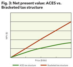
Figure 3 conceptually illustrates the potential difference directionally in net present value between tax structures where progressivity is bracketed and the ACES tax structure where higher tax rates apply to all previous dollars of value. In the latter the returns to the producers may be greatly contained at high prices.
High marginal tax rates can also create non-productive spending. Progressivity works in reverse as price goes down. As market price declines from $80/bbl to $79/bbl, 77 cents out of the decrease is realized by the government. Net value also declines as spending goes up, as well as when prices go down. So if prices are at $80/bbl, if there is an extra dollar of spending, again, the government realizes 77 cents less.
Insofar as the marginal tax represents what government gets as price goes up, it also represents what government gives up as either price goes down or costs go up. Regarding the latter, the marginal tax rate represents the government contribution to spending.
Thus high marginal tax rates create an incentive to "gold-plate," spending more than you ordinarily would because someone else is picking up most of the tab. Although the incentive is present whenever the extra value of an item exceeds the after-tax cost actually paid, the higher the marginal tax rate the more important this effect.
Curtailment of upside potential
Investment decisions for oil production activity depend, of course, on a myriad of factors, price being one of the most important. And oil price is notoriously volatile.
Accordingly, investment decisions are heavily cloaked in uncertainty. Thus rather than analyze a potential project at one price, investors will often look at performance over a range of prices. For many oil companies this will be conducted stochastically, often through a Monte Carlo, or similar simulation method.
In such practices, the input for price will consist of a distribution of expectations over a spectrum of probabilities. One such hypothetical distribution is shown in Figure 4.
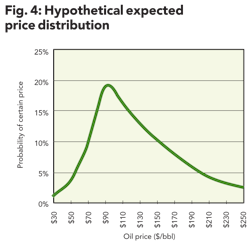
Such a shape for the distribution curve may not be atypical. For instance, the current US Department of Energy long-run forecast for annual price growth is -1% in the low case, +1% in the reference case, and +3% in the high case.
Where the most likely price (the mode), the one with the highest probability, may be $90, (the approximate current long-run consensus forecast), due to a number of factors reflecting price outlook, there may be higher probabilities price could be higher than $90 rather than lower. There is just more room and possible reasons for price to move up rather than down.
Hence, the curve is skewed to the right.
Investors would not focus on just the one price with the highest probability, but on the spectrum of prices. In this particular distribution the mode is $90, the median price is about $110, and the mean is about $130, both much higher than the $90, reflecting greater upside (high price) potential than downside (low price) potential. Investors would use the median or mode in their project analysis. They would not use the $90.
Consequently, what happens on the upside can have a dramatic effect on the expected result weighted over the entire distribution. If the upside (profit) potential is not suppressed it can markedly improve these expected results. Even if the upside potential is of relatively low probability, it represents an opportunity for a great deal of cash flow, and can have such a dramatic effect when it does occur that it can play a pivotal role in feasibility analysis. Thus the importance of upside potential should not be negated.
This is intensified by exploration risk. A serious exploration program may cost hundreds of millions of dollars, and there may be a 50% chance an explorer will come up dry and lose money. It takes a lot of upside potential to offset the high risk of losing large sums of money 50% of the time.
However, since the marginal tax rates are so high under Alaska's structure, the progressivity takes away much upside potential from producers.
Is the curtailment of upside potential balanced with commensurate sharing of downside price risk? As price falls the production tax rate goes down to the base rate of 25% of net value and then stops. Contrast this, for example, with the lowest federal corporate income tax rate of 15%. In competitive terms, as we will intimate in the International Comparison section below, Alaska's floor may not be a very low rate. Accordingly, the government does not share equitably in downside price risk. There is little risk symmetry.
The role of capital credits in tempering the asymmetry is modest. The credits will be a fixed amount regardless of price, juxtaposed against a high percentage of a large amount of value on the upside. The cash flow difference is substantial. (The production tax structure was initially devised in 2006, without progressivity, with international competitiveness as a design criterion, using a 5 percentage point difference between the tax rate and the credit rate. See Van Meurs.)
INTERNATIONAL COMPARISON:
TWO CASE STUDIES
Case study 1: ConocoPhillips worldwide operating results
ConocoPhillips (CP) is one of the three major working interest owners on the North Slope. (The others are BP and ExxonMobil.) Alaska constitutes a major portion of CP's assets, and it reports the result of their Alaska operations separately. (Other companies do not.) CP's operating results are presented in their Annual Report and Securities and Exchange Commission (SEC) Form 10-K.
Another way to get a perspective on upside potential is to compare the 2008 (the first full year ACES was in effect), and 2009 financial operating results for CP inside and outside Alaska. Oil prices in 2008 were high, peaking near $150/bbl and averaging nearly $100/bbl, and quite a bit lower in 2009, averaging around $60/bbl. By comparing what happens to taxes in high and low price years we can get a good picture as to how much upside potential is captured by taxes.
ConocoPhillips has a presence in over 30 countries, and by nearly any measure is one of the world's largest private (not state-owned) exploration and production companies. Their tax situation is a good representation of international tendencies, and a comparison between their Alaska and non-Alaska taxes provides a barometer of Alaska's relative tax picture.
CP's production in Alaska is nearly all crude oil (and natural gas liquids). Outside Alaska CP operations are about half oil and half gas. Their worldwide gas prices in 2008 and 2009 were $8.28 per thousand cubic feet (mcf) and $4.30/mcf, respectively.
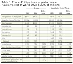
Table 3 shows ConocoPhillips reported operating results inside and outside Alaska for 2008 and 2009. (The figures include the results of natural gas operations, as well.)
In Alaska, where pre-tax income was $3,673 million higher in 2008, after-tax income was only $775 million higher. Only 21% of the additional pre-tax income was retained after-tax. About 80% of the additional taxes were non-income taxes, nearly all of which was the production tax.
Outside Alaska 51% of the pre-tax income was retained after-tax. This illustration would suggest the production tax significantly limits upside potential.
Case study 2: PFC Energy study
In October 2007 PFC Energy produced for the State of Alaska a publicly available report comparing worldwide government take. PFC's data set contains 190 of the largest international oil projects from 18 countries.
The report showed that at an $80 market price only 20% of the projects have higher marginal tax rates than Alaska. (The report was prepared prior to the run-up of prices in 2008, and $80 was the highest price examined.) The report also showed that the jurisdictions with higher marginal tax rates are areas under production sharing agreements, where resource potential is higher, the operating environment is lower cost/less harsh, and fiscal stability terms are available.
As far as downside price risk is concerned, PFC showed that at $30 only about 28% of the other worldwide projects have higher marginal tax rates than Alaska. This underscores the risk asymmetry discussed above.
Conclusion
Progressivity is an accepted and widely utilized instrument of taxation, and there is certainly a role for it. The philosophy is straightforward. At lower income there is less ability to pay taxes and there is a lower tax rate. At higher income there is more ability and there are higher rates.
The lowest dollars of value retain their diminutiveness regardless of what higher value ones follow. These dollars have a limited ability to pay taxes, and most jurisdictions in their tax structures protect these low dollars from progressivity through bracketing. In bracketing, only incremental value is subject to higher tax rates.
Alaska's production tax is unique in that there is no bracketing. When progressivity occurs it applies to the very first dollar of value, as well as all subsequent dollars. Thus as value increases, additional tax is extracted from all previous value.
This can create high marginal tax rates. At higher prices a large share of incremental value goes to the government, which can significantly suppress upside potential. Given the importance of upside potential in portfolio analysis, Alaska's international attractiveness for investment may be uncompetitive.
Many proposals have been floated within Alaska to address the effects of high marginal rates. However, most simply reduce the slope of the progressivity curve or create additional credits; few actually correct the underlying problem.
About the author

References
Alaska Department of Revenue, "Spring 2010 Forecast," p. 8. (http://www.tax.alaska.gov/programs/documentviewer/viewer.aspx?1943f)
ConocoPhillips, "2009 SEC Form 10-K", February 25, 2010, pp. 148-154. (http://phx.corporate-ir.net/phoenix.zhtml?c=132222&p=irol-sec&seccat01.1_rs=21&seccat01.1_rc=10)
Energy Information Agency, US Department of Energy, 2010 Annual Energy Outlook. (http://www.eia.doe.gov/oiaf/aeo/)
PFC Energy, "Government Take Comparison," a report prepared for the Alaska Department of Revenue, October 20, 2007, p.3. (http://www.revenue.state.ak.us/ACESDocuments/PFCenergy/pfc%20torsten%20legis%20slides.pdf)
Van Meurs, Pedro, "Proposal for a Profit Based Production Tax for Alaska," a report prepared for the State of Alaska Department of Revenue, February 14, 2006. (http://www.revenue.state.ak.us/gasline/ContractDocuments/Contractors/VanMeurs&Associates/CDP_703835.pdf)
More Oil & Gas Financial Journal Current Issue Articles
More Oil & Gas Financial Journal Archives Issue Articles
View Oil and Gas Articles on PennEnergy.com