Application of Markowitz portfolio theory in the oil and gas industry
Gary L. Cartwright, Devon Energy Corp., Oklahoma City
Modern portfolio theory is designed to optimize return for a given level of variance across a spectrum of investment opportunities. The ability to monitor and optimize a portfolio gives rise to the ability to manage a portfolio toward certain goals and objectives.
“The basic premise of portfolio theory is that the variance of returns for a portfolio of risky assets is a function not only of the variance of each individual asset, but also of the covariance [or correlation] between each asset (variance of return, or standard deviation of return, can be considered a measure of economic risk). When multiple risky assets are held within a portfolio, it can be expected that some properties will increase in value while at the same time others will decrease in value. By holding risky assets in groups, some of the risk of each asset may be reduced or eliminated through the process of diversification.
Additional potential arises from understanding the relationship among the respective projects relative to success or failure. If two projects are negatively correlated, i.e. if success in one project is associated with failure of the other, and failure in one is associated with success in the other, this significantly reduces the risk of double failure across the two projects. If independent, the full value of diversification is achieved; if negatively correlated, natural hedges reduce the risk of complete loss potentially to zero.”2
How then is variance or variability estimated for assets within a portfolio? The goal of portfolio diversification is to build wealth in the future; hence, knowledge of future variability would be the best criteria to estimate. However, the future is unknown and unknowable. Thus, portfolio managers must examine the past variability among assets as a means to estimate future variability.
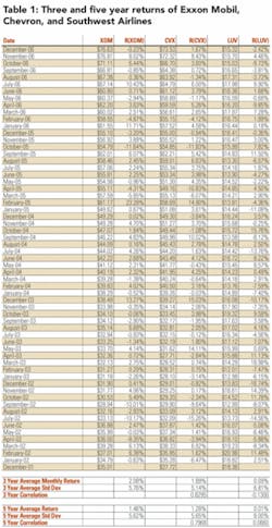
As an example of this methodology, consider the security performance of the three assets shown in Table 1, ExxonMobil (XOM), Chevron (CVX), and Southwest Airlines (LUV).3 Respectively, these securities represent the stock performance of two major oil companies and a passenger airline.
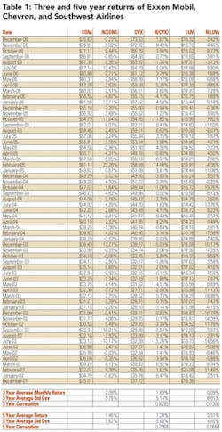
Without running through the calculations, intuition suggests that the returns of XOM and CVX are closely correlated and, hence, their correlation coefficient would approach 1.0. Both companies have wholly owned exploration and production subsidiaries as well as refining and marketing subsidiaries. Oil and gas commodity price increases and decreases should affect the companies similarly.
When commodity prices increase, the revenues of XOM and CVX increase, then prices go down, the revenues of XOM and CVX decrease. At the same time, intuition suggests that the returns of XOM and LUV would not be highly correlated and, hence, their correlation coefficient would substantially deviate from 1.0.
In contrast with XOM, oil and gas commodity price increases represent a cost increase to LUV, while for XOM it would represent a revenue increase. Similarly, a commodity price decrease would represent a cost decrease to LUV but for XOM it would represent a revenue decrease.
Table 1 provides the monthly return calculation for each of the three securities and how these return average and vary over a three and five year time horizon as measured through December 2006. Based on this analysis over the past three years, XOM has an average monthly return of 2.08% with a standard deviation of 5.76%; CVX has an average monthly return of 1.89% with a standard deviation of 5.14%; LUV has an average monthly return of 0.09% with a standard deviation of 6.81%.
The correlation coefficient measured between XOM and CVX during this period is 0.83, while the correlation coefficient measured between XOM and LUV is -0.13.
However, returns, variance, and covariance are not constant over time. Over the five-year period ending December 2006, XOM’s average monthly return is 1.46% with a standard deviation of 5.62%; CVX’s average monthly return is 1.28% with a standard deviation of 5.65%; and LUV’s average monthly return is 0.01% with a standard deviation of 8.00%.
The correlation coefficient measured between XOM and CVX during the five-year period is 0.80, while the correlation coefficient between XOM and LUV is 0.07. The hedging of their energy position served to dampen the variance of LUV’s cost, which was reflected in its stock price performance.
Table 1 validates the prior expectations between these three securities in that firms within the same industry (XOM and CVX) have a tendency to be more correlated in terms of security performance than firms from separate industries (XOM and LUV), especially where the revenue drivers of one industry are the cost drivers of the other.
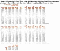
Combining two investments with correlation coefficients less than 1.0 can generate a portfolio return, which exhibit less variability for a given level of return. Table 2 and Figures 1 and 2 illustrate the reduction of variability for asset combinations of XOM and CVX and for XOM and LUV. Also, Table 2 uses the returns and variances derived over the most recent three years for the three securities.
Various weighting factors are combined for XOM versus CVX and for XOM versus LUV. The weighting factors range from -100% to 200% but always such that the sum of the two component weighting factors adds to 100%. This enables an evaluation of a short position in one of the securities relative to the other security during the time period being evaluated.
The standard deviation of the portfolio is shown as St Dev (Pf). The expected return of the portfolio is shown as Exp Return (Pf). For further illustration, the expected portfolio return for a weighting of 50% XOM and 50% CVX is 1.99% while its standard deviation is 5.22%; similarly for a portfolio of 50% XOM and 50% LUV, the expected portfolio return is 1.09% while the standard deviation is 4.17%.
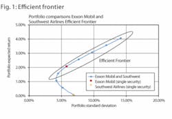
Figure 1 provides a graphical presentation of the XOM and LUV portfolio and introduces the “efficient frontier”4 concept. It shows the portfolio’s expected value as a function of the portfolio’s standard deviation. The efficient frontier is composed of those portfolio combinations, which result in the expected returns along the upper arm of the resultant curve. In other words, a rational investor would prefer a higher expected return to a lower expected return for the same level of risk. Thus, the upper curve of the expected value function forms the efficient frontier.
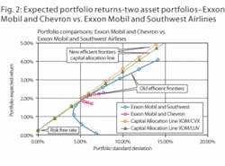
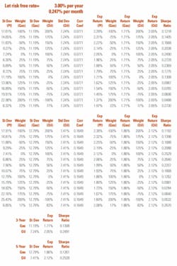
Figure 2 and Table 2 also introduce the concept of the Sharpe5 ratio and Capital Allocation Line.6 The capital allocation line is defined as the line formed by joining the tangency point of the efficient frontier and the risk free interest rate. For the purpose of this table and figure, a risk-free annual rate of 3.0% is assumed which translates to a 0.25% risk-free rate per month.
Based on the placement of the capital allocation line, the optimum mix of a pure equity investment can be defined as the point of tangency. For the XOM and CVX portfolio, this occurs at a 47% weighting of XOM and a 53% weighting of CVX. For this weighting, the portfolio yields an expected return of 1.98% and a standard deviation of 5.2%.
For the XOM and LUV portfolio, the point of tangency occurs at a weighting of 95% XOM and 5% LUV. This portfolio yields an expected return of 1.99% and a standard deviation of 5.45%. Utilizing the capital allocation line, the returns of both portfolios can be enhanced by borrowing funds and purchasing more of the portfolio. The return for this type of investment strategy would lie along the capital allocation line to the right of the tangency point.
On the other hand, the risk of the portfolio can be reduced by divesting of portions of the all equity portfolio and investing in the risk free asset; the risk and return for this type of investment strategy would lie along the capital allocation line to the left of the tangency point. The Sharpe ratio reflects the slope of the capital allocation line and represents the maximum expected return for the given level of risk or standard deviation.
Thus under modern portfolio theory, diversification can be accomplished by examining past behavior of security returns and determining how they vary over time and how they vary with respect to each other. This, of course, assumes that past return variance will be a reasonably good indictor of future variance. Armed with the knowledge of past behavior, an optimal equity portfolio position can be determined in relation to a capital allocation line. An investor can then determine his or her risk tolerance and return objectives and position the portfolio equity and debt risk accordingly.
As a cautionary note, however, not all risk is diversifiable.
“Economic risk can be considered in two parts; risk that is unique to a particular asset (unique risk) and, risk that is shared among all assets (systemic risk). The unique risk of an asset can be reduced through the diversification effects of holding multiple assets. The systematic component of risk is non-diversifiable. [Examples of systematic risk are general economic booms, recessions, and depressions.]
“To use portfolio analysis, it is necessary to determine the character of risk, i.e. its systematic and unique components. This is done [in part] by determining the expected return and variance of return for each asset, and the covariance of returns between the assets making up the portfolio. Once the nature of risk for each asset is determined, portfolio theory provides an analytical means for selecting the specific mix of assets which will optimize the entire portfolio’s risk-return relationship.”7
Oil and gas investment applications
Modern portfolio theory is based on the diversification of securities to achieve an optimal return for a given level of variance or uncertainty. Actually, the concept of diversification is not new to the oil patch. Ownership in oil and gas investments has typically been structured to permit the sharing of uncertainty or risk by multiple parties. Partial interests8 in wells have often been sold or traded to reduce the risk of a dry hole by any single company or individual. Intuitively, it is better to have a 50% interest in two wells with at 50% dry-hole risk than a 100% interest in one well with a 50% dry-hole risk.
However, a note concerning oil field jargon is appropriate here. Markowitz equates the term “risk” with “variance of return.” In oilfield terms, risk typically “denotes the possibility of a monetary loss or an unachieved objective.”9
Although, the term “risked investment” or “risked net present value” refers to the resultant single value of a decision tree analysis. Variance of return has a consistent meaning within the financial and oilfield worlds. However, risk, uncertainty, and probability have differing meanings across the oil industry. It is always a good idea to establish the proper context when discussing oilfield statistical analysis within the industry.
Although, diversification was not a new subject to the oil and gas industry, portfolio management and efficient frontier nomenclature did not enter oilfield jargon until the 1990s. Hightower and David10 introduced the concepts of modern portfolio theory to the oil and gas industry in 1991 in their paper, “Portfolio Modeling—A Technique for Sophisticated Oil and Gas Investors.”
If securities represent discounted future cash flows of a firm, then oil and gas assets can be thought of in a similar manner, which is simply to discount the expected cash flow from the oil and gas investment. In addition, if the variance of securities pricing can be equated to the variance of possible oil and gas investment outcomes, then we can apply the modern portfolio theory to oil and gas investments.
However, variance in securities portfolios are estimated from past securities return performance. While an estimate of oil and gas project variance can be gained from past performance, the more common practice is to create a stochastic model based on possible outcomes combined with a Monte Carlo simulation.11,12
The cashflow of a potential oil and gas project is shown in Table 3. The revenue of an oil and gas project is derived from its volume of oil and gas production, the commodity price of these components, the operating costs to maintain the oil and gas flow and the investment required to bring the project on line. Among the uncertainties or variances of the components are the ultimate volumes of the oil and gas that are known as oil and gas reserves, the price of oil and gas, the costs of operating the well, and the investment required for the project.
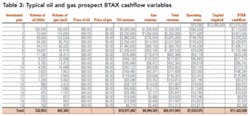
In Table 3, the reserves for the well are 332,953 barrels (bbls) of oil and 832,383 thousand cubic feet (mcf) of gas. Among the components of the cash flow, the oil and gas reserve and production flowstreams are the most variable, followed by the investment, the commodity pricing, and lastly the operating costs.13
Oil and gas pricing can be hedged through the purchase of futures contracts and/or swaps,14 investments can be estimated with reasonable certainty except during periods of rapid commodity price increase or decrease (boom and bust cycles).
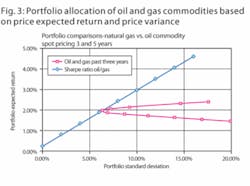
Absent price hedging to remove variance and uncertainty, a rationale investor can treat the variance of commodity pricing as a means of weighting a portfolio composed of oil and gas assets. Figure 3 illustrates the most recent three- and five-year commodity price performance of oil and natural gas. The analysis of Figure 3 is set up with the same assumption of a 3% risk free rate as utilized in Table 2 and Figures 1 and 2. Based on this type of analysis, a 23% natural gas and 77% oil portfolio yields the optimum Sharpe ratio based on the most recent three-year period.
null
null
Bibliography
- Markowitz, Harry. “Portfolio Selection,” The Journal of Finance, Vol. VII, No. 1, March 1952.
- Bratvold, R. B.; Begg, S. H. “Even Optimists Should Optimize”, SPE 84329, prepared for the SPE Annual Technical Conference and Exhibition held in Denver, Colorado, 5—8 October 2003.
- Historical stock prices sourced from http://finance.yahoo.com.
- Markowitz, op. cit.
- Bodi, Zvi; Kane, Alex; Marcus, Alan. Investments, McGraw Hill, 2005, p. 868.
- Sharpe, William F. “Capital Asset Prices: A Theory of Market Equilibrium under Conditions of Risk,” The Journal of Finance, Vol. 19, No. 3, September 1964, pp. 425-442.
- Edwards, R.A.; Hewett, T.A. “Applying Financial Portfolio Theory to the Analysis of Producing Properties”, 68th Annual Technical Conference and Exhibition of the Society of Petroleum Engineers held in Houston, Texas, 3-6 October, 1993.
- MacKay, James A. “Utilizing Risk Tolerance to Optimize Working Interest”, SPE 30043, prepared for presentation at the SPE Hydrocarbon Economics and Evaluation Symposium, Dallas, Texas, 26-28 March 1995.
- Campbell, J.D. Analysis and Management of Petroleum Investments: Risk, Taxes, and Time, 2nd Ed., CPS Publishing, Norman, OK, 1991.
- Hightower, M.L.; David, A. “Portfolio Modeling: A Technique for Sophisticated Oil and Gas Investors,” Society of Petroleum Engineers, SPE 22016. Presented at the SPE Hydrocarbon Economics and Evaluation Symposium in Dallas, Texas, 11-12 April 1991.
- Edwards, R.A.; Hewett, T.A., op. cit.
- Brashear, J.P.; Becker, A.B.; Faulder, D.D. “Where Have All the Profits Gone? Or, Evaluating Risk and Return of E&P Projects”, Society of Petroleum Engineers, SPE 63056, 2000 SPE Annual Technical Conference and Exhibition held in Dallas, Texas, 1-4 October 2000.
- Thompson, R.S.; Wright, J.D. Oil Property Evaluation, Thompson-Wright Associates, Golden, Colorado, 1985, p. 1-3.
- McDonald, Robert L. Derivatives Markets, 2nd Edition, Pearson Education, Inc., 2006, pp. 912-918.

Gary Cartwright [[email protected]] is corporate portfolio advisor for Devon Energy Corp. in Oklahoma City. He holds a bachelor’s and an MBA degree from the University of Oklahoma and a law degree from Oklahoma City University College of Law. Cartwright has work experience in reservoir engineering and drilling engineering for Exxon Corp., Texas Oil and Gas/Marathon Oil, and Enron Oil and Gas/EOG Resources. He has been with Devon since 2006.