CORROSION— Conclusion: Pitting corrosion models improve integrity management, reliability
New deterministic and stochastic models for external pitting corrosion in underground pipelines can help improve integrity and reliability analyses. This concluding article applies these models to Monte Carlo-simulated and real pipeline pitting corrosion data obtained from field and in-line inspections (ILI).
Part 1 of this series (OGJ, July 20, 2009, p. 64) described a deterministic predictive model relating pit growth to soil and pipeline characteristics, showing it is possible to establish a physically sound correlation between pitting model parameters and soil and pipeline characteristics.
Part 1 also described a continuous-time, nonhomogenous linear growth Markov process developed for stochastically modeling external pitting corrosion in buried pipelines, showing this type of Markov process to be particularly suitable due to the existence of a closed form solution to the system of Kolmogorov’s forward equations.1
Part 1’s results show Monte Carlo simulations effectively predict the probability distributions of soil corrosion pitting depth and rate. The complexity and cost of the necessary field and laboratory studies would otherwise prevent obtaining this information. The probabilistic description of corrosion pitting can realistically estimate the reliability evolution of cathodically protected, coated pipelines, for which the worst-case corrosion rates commonly recommended in the pipeline-corrosion literature might be exceedingly conservative.2-5
This article first applies Part 1’s deterministic pitting corrosion model to experimental data obtained through ILI and field inspections. A second example applies the pitting corrosion rate distribution obtained in Part 1 to data obtained from repeated ILI. A final example uses Part 1’s Markov chain model to predict the time evolution of pit-depth distribution in underground pipelines from soil properties. These examples show how the proposed models help improve pipeline integrity and reliability analyses.
Example 1
This real-life example involves integrity assessment of a coal tar-coated 62-km long underground oil pipeline with a 914-mm OD and an 11-mm WT. Magnetic flux leakage (MFL) ILI inspected the pipeline in 1997, after 18 years of service. Time-to-failure by leakage due to external corrosion pitting provided the basis for a remaining-life estimate. The ILI report and field inspections identified pits as corrosion-caused metal losses with diameter ≤ WT × 2. This same criterion applies to all case studies presented hereafter. A methodology developed by the authors calibrated the ILI reports (OGJ, Sept. 13, 2004, p. 76).6
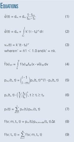
The first stage of ILI-based integrity analysis used the linear pit-growth model, assuming pits began to grow when the pipeline was commissioned (t0 = 0). The (constant) growth rate ascribed to each pit was determined as the ratio of each pit’s measured depth (dm) to the length of the time interval between the time of inspection (tILI) and the pipeline’s commissioning time (tC) determined the (constant) growth rate for each pit. Therefore, pit depth at any future time can be estimated with Equation 1.
A second stage of analysis used the prediction model for pit growth proposed in Part 1. Equation 2 computed the time evolution of the depth of the observed pits.
This stage integrated the pit growth rate defined by Equation 3 over the interval from tILI to t. The parameter values of Table 1 for the all soil category (t0 = 2.88 years, k’ = 0.128 mm yr-1/0.220, and n´ = -0.220) evaluated Equation 2 for each pit, modeling the pit growth using typical soil conditions observed for all collected samples.
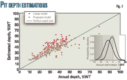
Repairs followed ILI and many sections of the pipeline were excavated and rehabilitated when necessary. This process measured the depths of a total of 123 pits detected at in-danger pipeline sections in the field. Exposure time for these pits ranged between 19 and 26 years. Fig. 1 plots the pit-depth estimates obtained with the linear growth model (Equation 1) and the proposed growth model (Equation 2) against the pit depths measured in the field (actual depths).
The estimations of both the linear and the proposed growth models show random errors always associated with this type of comparison plot. The perfect match (1:1) line in Fig. 1 shows, with respect to field-measured depths, linear model-based estimations are biased toward larger depths on average. The observed overprediction is considerably higher for the linear growth model than for the proposed model. The linear trend assumed for pit growth in Equation 1 leads to more conservative predictions than the power law trend in Equation 2, explaining the magnitude of the difference in overprediction, particularly when estimations cover relatively long time periods.
The inset in Fig. 1 shows the normal distributions fitted to the residuals obtained for both types of estimations, demonstrating that in addition to a reduction in the large overprediction produced by the linear model, application of the proposed pit growth model also allows for reduction of the uncertainty (scatter) in the estimations. Environmental differences between the observed pipeline and the all soil category explain the relatively small remaining overprediction seen during application of the proposed model.
The increase in accuracy and precision of pit-depth estimations produces a longer predicted remaining life for the pipeline and thus fewer scheduled repairs. In this example, even when the typical (average) soil conditions observed for all collected samples were used, a positive impact on integrity management occurred. Collecting the actual soil and pipe characteristics at each exposed pipeline section would likely further improve the accuracy and precision of maximum pit-depth estimations.
Example 2
The second real-life example involves estimation of the reliability trend of a coal-tar-coated, 82-km underground pipeline transporting sweet gas. The pipeline OD and nominal WT measured 355.6 mm and 9.52 mm, respectively. MFL-ILI inspection of the pipeline, commissioned in 1981, took place in 2002 and 2007. Fig. 2 shows the results of these inspections, presenting distributions of the estimated true depths of identified pits. Calibrating the ILI reports with a methodology developed by the authors yielded these distributions (OGJ, Sept. 13, 2004, p. 76). Fig. 2 also shows generalized extreme value (GEV)6 distributions fitted to the calibrated pit-depth data.
Assuming the soil properties along the pipeline to be similar to those observed for all collected samples allowed use of the time-independent long-term probability distribution of the pitting corrosion rate for the all soil class (ƒ(v)all) (last row in Table 2). A preliminary prediction, in which the GEV distribution fit to the ILI-derived pit depth distribution for 2002 (ƒ(x)02) was used to predict the pit-depth distribution for 2007 (ƒ(x)07), tested the suitability of this selection. This prediction used a time interval (δ) between the two inspections of 5.5 years (Equation 4).
Fig. 2 shows the predicted pit-depth distribution for 2007 (ƒ(x)02). It is close to the 2007-ILI-measured pit depth distribution and to the corresponding GEV fitted distribution, supporting the use of the long-term pitting rate distribution associated with the all soil class to predict the evolution of pipeline reliability with time.
After corroboration of the suitability for reliability estimations, (ƒ(x)07)(ƒ(v)all) estimated the time evolution of pipeline reliability over a 15-year period, beginning in 2007. For the sake of comparison, a second estimation used the pit growth-rate distribution (ƒ(v)lin) estimated with a linear pit-growth model. Assuming pits began forming upon pipeline commissioning yielded this estimation from the 2007-ILI pit depth distribution. A detailed description of the estimation of ƒ(v)lin lies elsewhere.7
Standard reliability methods predicted the time evolution of the pipeline’s annual failure rate/km-year with regard to corrosion-pitting-caused leakage failures (OGJ, Jan. 6, 2003, p. 54; OGJ, Jan. 13, 2003, p. 56). Fig. 3 shows the results of the reliability estimations conducted with ƒ(v)all and ƒ(v)lin. The reliability estimates obtained with f(v)all are much less conservative than the estimates based on the pitting rate derived from the linear pit-growth model. Over the time span considered (2007-22), the annual failure rate predicted with ƒ(v)all is, on average, three times smaller and increases much more slowly than that predicted with f(v)lin.
If these results were to be used for inspection planning based on a given reliability level of 1-(5 × 10⁻³/km-yr), an optimal reinspection interval of about 6 years would be predicted from the results of the reliability estimation based on the linear pit growth model. Using the long-term pitting rate for all soils from this study, by contrast, would produce a reinspection interval of about 12 years, demonstrating that a pipeline reliability model based on the long-term pitting rate distributions proposed in this work will realistically predict longer pipeline remaining life, longer reinspection intervals, and fewer unnecessary repairs compared to a reliability model based on the commonly used linear pit growth model.
Example 3
This example uses the proposed Markov chain modeling framework for pitting corrosion proposed in Part 1 to predict the evolution in time of pit-depth distribution in the all soil category. Researches set the initial damage distribution (pm(ti)) equal to the 10-year Monte Carlo-simulated pit-depth distribution in the all soil class. Equations 5-7 yielded the expected pit-depth distribution pl(t) for different future moments in time. The values of the parameters t0, n, and k were set equal to those in Table 1 for the all soil category.
Fig. 4 shows the results of these estimations, where the histograms represent the Monte Carlo-simulated pit-depth distributions and the continuous red lines represent the Markov chain-predicted distributions, pl(t). The proposed Markov chain model can accurately reproduce the time evolution of pit-depth distribution. The quality of fitting in the other soil classes was similar to the one presented here.8 The model can reproduce the changes observed in the shape of the pitting depth distribution over the entire estimation interval.
Part 1 of this article noted any of the three extreme value distributions (Weibull, Frechet, or Gumbel)6 could arise as the best fit to the pitting depth data in the investigated soils depending on exposure time, while the starting distribution is unique for each soil class. The proposed Markov chain model, however, adequately reproduces the variation in the shape of the Monte Carlo-simulated pit-depth distributions in all soil categories, from the beginning of the corrosion pitting damage process through the entire time span considered.
Another application of the proposed Markov chain model estimated the expected 2007 pit-depth distribution in the pipeline from the preceding example from the results of the 2002 ILI run. The empirical depth distribution observed in 2002 (Fig. 2) acted as the initial distribution (pm(ti)) in the Markov chain-based estimation. WT divided in 0.1-mm-thick states represented the corrosion pitting damage through a Markov chain with N = 100 states. The ratio of the number of pits with depths in the m-th state to the total number of pits observed during the 2002 inspection provided estimated probabilities (pm (ti).
Given pipeline commissioning in 1981 with soil characteristics assumed to be those of the all category, the values of the parameters necessary to conduct the estimation were: ti = 21 years, t0 = 2.9 years, n = 0.780, and t = 26.5 years (Table 1). The histogram in Fig. 5 represents measured pit-depth distribution in the pipeline for mid-2007, while the Markov chain-predicted pitting depth distribution, obtained with Equations 5-7, is shown with a thick red line. The particular shape of the Markov chain-estimated pit-depth distribution in Fig. 5 stems from the discrete nature of the Markov chain estimations as well as the discrete character of the pit-depth variable and its initial distribution pm(ti).
The high level of agreement between the empirical pit-depth distribution observed in 2007 and the Markov chain-modeled distribution also points to the accuracy of the proposed model. Validation of its ability to correctly estimate the evolution of the pit-depth distribution in the studied pipeline points to the viability of using the proposed model to predict the time evolution of the pitting rate and pipeline reliability over a given time.
Fig. 6 shows the corrosion rate distribution ƒ(v ;ti,t) associated with the entire population of pitting defects 2002–2012, obtained with Equations 8 and 9. The obtained pitting rate distribution is close to a GEV distribution with a shape parameter negative yet also close to zero. Either the Weibull or the Gumbel subfamilies of the GEV distribution, therefore, seem appropriate for describing the pitting rate in the pipeline over the selected estimation period.
One advantage the Markov chain approach has over deterministic and other stochastic models for pitting corrosion is its ability to capture the dependence of pitting rate on pit depth and lifetime. It allows for an estimation of not only the probability distribution of the pitting rate associated with the entire pit population (Fig. 6), but also the pitting-rate distribution for any subpopulation within specific lifetime and depth ranges.
Model limitations
A more complete predictive pit-growth model would incorporate microbial corrosion’s role, notably the effects of sulfate-reducing bacteria, as well as seasonal fluctuations in soil properties and their influence on the pitting damage process. The results described in this article apply to corroding pipelines in contact with clay, clay loam, and sandy clay loam soils in tropical regions. Caution should be exercised when applying the results to pipelines in contact with these textural classes in nontropical climates.
References
- Parzen, E. “Stochastic Processes, Classics in Applied Mathematics,” Society for Industrial and Applied Mathematics (SIAM), Philadelphia, 1999.
- Peabody., A.W. “Control of pipeline corrosion,” second edition, edited by Bianchetti, R., NACE International, Houston, 2001.
- ANSI/NACE Standard RP0502-2002, “Pipeline external corrosion direct assessment methodology,” NACE International, Houston, 2002.
- B31.8S-2004: “Managing system integrity of gas pipelines,” ASME Code for Pressure Piping, ASME, New York, 2008.
- Race, J.M., Dawson, S.J., Stanley, L.M., and Kariyawasam, S., “Development of a predictive model for pipeline external corrosion rates,” Journal of Pipeline Engineering, Vol. 6, No. 1, pp. 15-29, March 2007.
- Coles, S., “An Introduction to Statistical Modelling of Extreme Values,” Springer Series in Statistics, Springer-Verlag, London, 2001.
- Caleyo, F., Velazquez, J.C., Valor, A., and Hallen, J.M., “Probability distribution of pitting corrosion depth and rate in underground pipelines: A Monte Carlo study,” Corrosion Science, May 15, 2009.
- Caleyo, F., Velazquez, J.C., Valor, A., and Hallen, J.M., “Markov chain modelling of pitting corrosion in underground pipelines,” Corrosion Science, June 14, 2009.
