Stacked deep learning models predict cogeneration unit gas emissions
Yu Pang
Ling Bai
VL Energy
Calgary, Canada
Charles Grimm
Suncor Energy
Calgary, Canada
Marc Godin
Petroleum Technology Alliance Canada
Calgary, Canada
The shift towards AI-powered predictive emissions monitoring systems (PEMS) is seen as the future of gas emission monitoring due to its potential to accelerate digital transformation, reduce capital and operating costs, mitigate downtime, and enhance efficiency and productivity. A gas emission monitoring case study used a deep-learning-powered PEMS to predict and multivariate gas emissions from cogeneration units.
VL Energy performed a cloud-based and AI-powered PEMS study on Suncor Firebag’s Cogeneration Unit 194 (CG-194) in Alberta, Canada. The system forecast NOx, flow rate, and flue gas temperatures at the exhaust stack of the unit. PEMS matched measured data and met regulatory requirements.
The study shows that PEMS accurately predicts multivariate gas emissions from large stationary combustion sites and is a viable alternative for continuous emissions monitoring systems (CEMS) in the oil and gas industry.
CEMS-PEMS
Gas emissions are major contributors to global warming and air quality deterioration.1 To ensure compliance with regulatory emission limits, large stationary emission-source combustion sites typically use one or more CEMS to monitor gas emissions.2 Hardware-based CEMS are relatively expensive, however, and require frequent maintenance.3 In addition, CEMS cannot guarantee data availability during downtime and maintenance.4 Alternative methods, therefore, are required to continuously monitor gas emissions while reducing costs of operations and maintenance.
Unlike CEMS hardware dependency, PEMS is a software-based solution. PEMS technology can be segmented into three categories: first principles-based modeling, statistical-regression, and machine learning-based modeling.5 First principles-based models employ fundamental physical laws (e.g., mass balance and energy conservation) to calculate emissions. In contrast, statistical regression models establish correlations between operation parameters and emissions of combustion devices, constructing empirical models for prediction. Machine-learning (ML) models train predictive models based on operational parameters and emission datasets, offering greater flexibility and adaptability to new data and features. Therefore, ML-based models are advantageous in complex, non-linear systems where simpler models may struggle.
Incorporating ML-DL (machine learning-deep learning) into PEMS significantly boosts predictive accuracy and operational efficiency. Notably, PEMS incurs about 50% lower capital costs and 10-20% of the operational and maintenance expenses of CEMS.5 6 PEMS also offers real-time monitoring and prediction with minimal downtime, ensuring continuous data availability and aids users in optimizing operations while complying with environmental standards. It adapts to changing conditions and is implemented faster with less complications. Globally, several countries, including the US, Canada, Europe, Australia, and Singapore, have recognized PEMS as a viable gas emissions monitoring tool.7
VL Energy Ltd. performed a cloud-based and AI-powered PEMS study in a cooperative project with Suncor Energy Inc. The PEMS consisted of a collection of DL models which forecast emitted flue gas NOx concentration, mass flow rate, and temperature. The system was tested on Suncor Firebag’s CG-194 in Alberta. Performance was evaluated under normal and shutdown conditions, demonstrating compliance with Alberta’s CEMS standards.
Model development
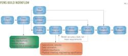
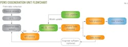
For PEMS projects, it is common to collect more than 100 distinct sensor tags (sensor readings) directly from the target combustion device. In general, such sensor readings include temperature, pressure, flow rate, moisture, etc., providing insights into the operational process and condition of the target device. Accordingly, a deep-learning-powered PEMS is built following data collection and preprocessing, feature engineering, model training, and model evaluation. Fig. 1 shows the workflow of building the DL model for PEMS. The blue components outline the systematic approach in a machine learning project, the green component signifies checkpoints for data quality, and the orange component checks focus on feature-related considerations.
Data preprocessing ensures robustness and resilience of the developed DL models in PEMS. Model development begins with the collection of extensive raw data, ranging from weeks to years, from physical sensors. Such data convey sufficient detail to characterize variations due to operational changes, maintenance activities, and environmental conditions.
The initial phase involves data cleaning and preprocessing to maintain data integrity and relevance. This includes verifying data type and pattern for consistency, analyzing data distribution to understand statistical properties, and identifying and rectifying outliers, noise, and missing values. Notably, data from device startup and shutdown periods, typically linked to maintenance, are retained to ensure model accuracy across varying operational states. Subsequently, the dataset is divided into training, validation, and test subsets. Feature selection, based on the training set, considers data volume and velocity, ensuring scalability and real-time processing. Correlation and significance analysis determine relevance of each attribute to predictive outcomes while also ensuring their engineering significance within the domain knowledge.
Subsequent models are constructed to simultaneously predict flue gas NOx concentration, mass flow rate, and temperature variables for specific combustion devices, while also detecting and correcting sensor failures and drifts. A variety of DL-ML algorithms are employed, stacked, and validated through this process, with hyperparameter optimization for each.
The validation dataset assesses model performance, guides model selection, aids hyperparameter tuning, and prevents overfitting. If a model fails to meet accuracy standards or desired performance levels, the feature selection stage is revisited. This iterative process continues until the model satisfies all criteria. Finally, the test dataset provides an unbiased evaluation of the model's performance. Rigorous testing and validation ultimately determine the best-performing model for deployment. This comprehensive approach ensures the development of accurate and reliable PEMS models.
PEMS model architecture
Steps from feature selection to model evaluation build all the models in PEMS (Fig. 1). This PEMS contains four DL models to predict NOx concentration, mass flow rate, and temperature of flue gas, and handle sensor failure and drift. The four DL models can work both independently and in parallel after deployment.
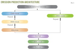
Fig. 2 shows the architecture of stacked DL models. This DL architecture integrates several key components: convolutional neural network (CNN) blocks, recurrent neural network (RNN) blocks, attention layer, and artificial neural network (ANN) blocks. These elements are specifically structured to effectively process and interpret both time-series and structured datasets. In terms of the PEMS projects, most operating parameters of combustion devices are categorized as time-series data (sensor readings), notable for their sequential nature and temporal relevance. Conversely, operating settings of these devices are classified as structured data, systematically arranged in a tabular format with clearly defined rows and columns.
The left-hand branch in Fig 2 consists of the CNN blocks, RNN blocks, and attention layer. The successive CNN blocks extract features from sequences. The outputs of the CNN blocks are sent to RNN blocks, and the successive RNN blocks capture complex temporal dependencies in sensor readings. Next, an attention layer is added to focus on important features in the sequence and capture long-range dependencies.
ANN blocks, which are designed to process the structured features, form the right-hand branch of the architecture. The outputs of left-hand and right-hand branches concatenate into a long array containing all sequential and tabular features and are then sent to a dense layer to obtain the final output. It should be noted that the weights, activation function, and repeat times for the CNN unit, RNN unit, and ANN unit are determined and optimized using the grid search technique.
Sensor failure, drift
Fig. 3 outlines the process for identifying sensor failures and drifts. The procedure uses the developed models for accurate prediction of future sensor readings and leverages historical data for identifying sensor anomalies.
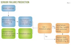
To predict sensor readings, algorithms such as XGBoost, Random Forest, ANN, and RNN develop predictive models for key sensors. Among these, models exhibiting the highest accuracy are chosen as the final predictive models for target sensors. These predictions are then juxtaposed with actual sensor readings to discern significant discrepancies. This comparison incorporates statistical analysis, comparing mean values of predicted and actual sensor readings within a set interval, determined by the sensors' reading frequency. This method is specifically designed to reduce false discrepancies from occasional data point deviations.
Data scientists and process engineers review sensor readings from past months or years to label sensor failure or drift and to define threshold values for each target sensor. When the discrepancy between predicted and actual readings surpasses the threshold value, the system activates an alarm or flag for sensor anomalies. Subsequently, it automatically backfills the measured sensor values with the predicted ones. This enables the DL models, used for forecasting NOx concentration, mass flow rate, and flue gas temperature, to recalibrate their forecasts using the backfilled sensor data, thereby enhancing the system's reliability and accuracy.
Suncor Energy cogeneration unit
Firebag field, 120 km northeast of Fort McMurray, Alta, produces as much as 215,000 bo/d from about 600 wells. Key to its efficiency are five cogeneration units, which together generate about 425 Mw of electricity with low greenhouse gas (GHG) intensity. This cogeneration system, fueled by natural gas, efficiently produces both industrial steam and electricity in the least GHG-intensive hydrocarbon-based method available. Additionally, excess power from these units is supplied to Alberta's electricity grid, contributing to a reduction in the province's carbon footprint.
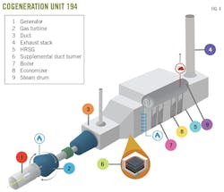
Fig. 4 shows CG-194, a principal emission source in the PEMS application. This unit, comprising a generator, gas turbine, duct, exhaust stack, heat recovery steam generator (HRSG), and supplemental duct burner, primarily generates electricity and heat. Due to its significant role in emissions, this cogeneration unit is equipped with a CEMS to monitor and report flue gas NOx concentration, mass flow rate, and temperature at the exhaust stack. Additionally, it features about 160 physical sensors, especially on the gas turbine and HRSG, to gather critical operational data, ensuring performance efficiency and environmental compliance. This extensive sensor network is engineered to capture a wide array of operational data, crucial for monitoring the unit's performance.
PEMS
Fig. 5 illustrates the structure and workflow of the developed cloud-based and ML-DL PEMS for CG-194. The PEMS comprises three main modules: the data pipeline module (orange components), the DL-ML module (green components), and the user interface module (blue components). The data pipeline module contains a flow path for collecting, transforming, and moving data from diverse sources to DL-ML models, data storage, and data analytics systems, and finally to the user interface.
The DL-ML module includes functions for predicting gas emissions for cogeneration during working- and off-states as well as sensor failure detection and correction. It also contains a continuous integration and continuous deployment (CI-CD) pipeline, automatically redeploying updated or retrained DL-ML models to the PEMS in accordance with the outcomes of the relative accuracy test audits (RATA) test. In addition, the user interface module is designed for client interaction, displaying comprehensive data analyses, predictions, and monitoring results.
For the DL-ML module, PEMS models for predicting NOx concentration, mass flow rate, and temperature at the exhaust stack of the cogeneration unit were trained, validated, tested, and further blind-tested based on data from 2017 to 2023. Data from January 2017-January 2020, February 2020-December 2020, January 2021-August 2022, and September 2022-March 2023 were assigned as training, validation, testing, and blind testing datasets, respectively. After data preprocessing, about 3 million data points were compiled to develop the model. Limiting input attributes and features to less than 20 managed computational resources more effectively and facilitated easier data collection and preprocessing, optimizing overall performance and efficiency.
Fig. 5 also displays the data collection process (dark blue components) on site. It includes 130 quality-assured sensors to measure parameters reflecting the operational status of the cogeneration unit. Data are recorded every minute via the distributed control system (DCS) and subsequently aggregated into the enterprise data control system for storage and future use.
Model results
The table summarizes the performance of the developed DL models. These models were evaluated using R-squared (R2) and root mean square error (RMSE) metrics in accordance with the CEMS code in Alberta. According to the code, the R2 obtained from comparing PEMS testing data with actual measured CEMS data must be equal to or greater than 0.64.8 R2 for the three DL models exceed 0.9, surpassing the minimum requirement. R2 from blind testing exceeded 0.87, reinforcing the robustness and reliability of these DL models in practical applications.

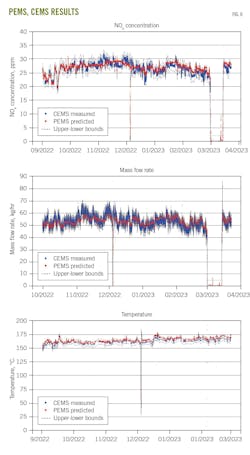
The PEMS predictions align closely with CEMS measurements for CG-194 in both operational and non-operational states. Moreover, the PEMS predictions fall within the upper and lower bounds defined by CEMS data, further validating the feasibility of PEMS in practical emission monitoring scenarios.
References
- Fiore, A. M., Naik, V., and Leibensperger, E. M., “Air quality and climate connections,” Journal of the Air & Waste Management Association, Vol. 65, No. 6, May 15, 2015, pp. 645-685.
- US EPA, “An Operator’s Guide to Eliminating Bias in CEM Systems,” No. EPA/430/R-94-016, 1994.
- Ciarlo, G., Bonica, E., Bosio, B., and Bonavita, N., “Assessment and testing of sensor validation algorithms for environmental monitoring applications,” Chemical Engineering Transactions, Vol. 57, Mar. 20, 2017, pp. 331-336.
- Chien, T. W., Chu, H., Hsu, W. C., Tseng, T. K., Hsu, C. H., and Chen, K. Y., “A feasibility study on the predictive emission monitoring system applied to the Hsinta power plant of Taiwan Power Company,” Journal of the Air & Waste Management Association, Vol. 53, No. 8, 2003, pp. 1022-1028.
- Si, M., Tarnoczi, T. J., Wiens, B. M., and Du, K., “Development of predictive emissions monitoring system using open-source machine learning library–keras: A case study on a cogeneration unit,” IEEE Access, Vol. 7, July 24, 2019, pp. 113463-113475.
- Chien, T. W., Hsueh, H. T., Chu, H., Hsu, W. C., Tu, Y. Y., Tsai, H. S., and Chen, K. Y., “A feasibility study of a predictive emissions monitoring system applied to Taipower’s Nanpu and Hsinta power plants,” Journal of the Air & Waste Management Association, Vol. 60, No. 8, 2010, pp. 907-913.
- Neto, A. S. A., Secchi, A. R., Capron, B. D., Rocha, A., Loureiro, L. N., and Ventura, P. R., “Development of a predictive emissions monitoring system using hybrid models with industrial data,” Computer Aided Chemical Engineering, Vol. 51, 2022, pp. 1387-1392.
- Alberta Environment and Parks, “Continuous Emission Monitoring System (CEMS) Code,” Apr. 4, 2021.
Authors
Yu Pang ([email protected]) is a senior data scientist at VL Energy specializing in integrating machine learning with petroleum engineering and environmental science. He holds a Ph.D. (2017) in petroleum engineering from Texas Tech University. He is an active member of SPE and ACS.
Ling Bai ([email protected]) is the CEO of VL Energy. He holds an MS (2018) from the University of Calgary. She is affiliated with the Clean Resource Innovation Network (CRIN), Innovate Calgary, Air & Waste Management Association, and Petroleum Technology Alliance Canada (PTAC).
Charles Grimm ([email protected]) is an environmental and regulatory advisor at Suncor. He holds a BS (2013) from the University of Calgary. He is affiliated with the Environmental Careers Organization of Canada and the Air & Waste Management Association.
Marc Godin ([email protected]) is the director of technology at Petroleum Technology Alliance Canada (PTAC). He holds an MBA (1986) from the University of Calgary. He is affiliated with the Petroleum Technology Alliance Canada (PTAC).