Unnecessary & avoidable mistakes in financial calculations

Financial mistakes can be inadvertent or they can be solely due to lack of command over the subject matter. Some mistakes can be fatal and some may be trivial but embarrassing. Whatever the cause or magnitude of mistakes; they are unnecessary and should be avoided. The irony is that such mistakes are committed by experienced analysts and not necessarily by amateurs.
M. A. Mian, Saudi Aramco, Dhahran, Saudi Arabia
The purpose of this article is to highlight some of the most common misconceptions in financial calculations. The examples provided are not hypothetical. They represent real-life situations encountered by the author and therefore, it is considered prudent to share them with others in the industry.
Management is normally exposed to making capital budgeting decisions based on single profitability indicators such as Net Present Value (NPV) or Rate of Return (ROR), etc. If the methodology used to arrive at these profitability indicators is incorrect or does not mirror real-life situations then the management decision will be in error.
In my opinion, two main sources are responsible for misconceptions and mistakes in financial analysis. One is Microsoft ExcelTM. This powerful tool, with its built-in financial functions, has revolutionized financial calculations. The problem however, is that anyone who can use the financial functions of Excel now claims to be a financial analyst, economist, or investment evaluation expert. This article shows that using Excel’s capability without logic and common sense could lead to fatal and/or embarrassing mistakes. The second source is financial textbooks and literature. Most avoid mirroring real-life situations. When analysts indiscriminately use textbook examples to represent real-life problems, they end up committing mistakes.
An article entitled “Revisiting the Pitfalls and Misuse of WACC” appeared in the October, 2005 issue of the Oil & Gas Financial Journal. This article showed some common mistakes committed by experienced analysts, including the financial effects of an investment in the discount rate and at the same time in the cash flows and/or considering that Capital Asset Pricing Model (CAPM) and WACC are synonyms. These misconceptions are due to ignorance and lack of adequate command over the subject matter.1
The Time Zero assumption
This assumption in financial analysis has created much confusion. The discounted cash flow (DCF) approach is the primary technique of investment/project evaluation and capital budgeting process. This approach requires forecasting detailed cash flow of the project under evaluation and then discounting the resulting cash flow to the present value (Net Present Value - NPV) using an appropriate discount rate. The following equation, for NPV calculation, is typically presented in most financial textbooks.2

where
NCFt = Net cash flow at time t
I0 = Investment (negative) at the beginning of the first year of project
i = Appropriate discount rate (fraction), i.e., cost of capital
In practice, the actual time zero may not be the beginning of the first year of the project/investment. The time zero is usually a common date, like 01/01/2006, at which the NPV of each prospective project in a planning period is calculated. Some of these prospective projects may start a year or more later than the time zero, like 01/01/2008, etc.
Furthermore, not every project under evaluation will have instantaneous layout of investment at the beginning of the first year of the project. This assumption is mostly valid for projects that do not require longer implementation periods. Most major projects will require three to four years of construction period and the expenditure will be disbursed periodically over each year. Therefore, inappropriate treatment of the initial investment may be detrimental to the NPV of the project. In addition, the future cash flows of a project are also received throughout the year, but in the cash flow they are assumed to be received at the end of the year.
Once the net cash flow of the project is obtained, Excel’s financial function “=NPV(rate,value1,value2,...)” is used to calculate its NPV. This function assumes that “value1, value2,...” are equally spaced in time and occur at the end of each period.

The NPV investment begins one period before the date of the value1 cash flow and ends with the last cash flow in the list. The NPV calculation is based on future cash flows. If the first cash flow occurs at the beginning of the first period, the first value must be added to the NPV result, not included in the values arguments. Some of Excel’s financial functions, such as PV, allow cash flows to begin either at the end or at the beginning of the period. Any blank cell in the array of cash flows will not be counted in the total number of years of the project and result in incorrect NPV; zero must be entered in these blank cells.

The description of the NPV function seems to be simple and straightforward. However, it can lead to fatal mistakes if one uses it without paying adequate attention to the structure of the cash flow. One such mistake, a real case, is shown in Table 1.
An analyst performs lease versus buy economics and develops a cash flow similar to the one shown in Table 1. An analyst religiously follows Equation (1) and enters Excel functions “=NPV(B3,C9:F9)+B9” and “=NPV(B3,C18:F18)+B18” in Cell-B20 and Cell-B21 to calculate the NPV of lease and buy options, respectively. However, the analyst fails to pay attention to the various values in Column B, thus resulting in a fatal mistake. In order to visualize the mistake, the financial function entered in Cell-B21 is translated into a time diagram as shown in Figure 1.
The NPV function in Cell-B20 can also be translated into a time diagram to visualize the cash flows. The following points are illustrated by Figure 1.
1. The first interest and principal payments are made on the same day as the loan withdrawal. Similarly, interest tax advantage has been availed on the day the loan is withdrawn. The second and subsequent payments start two years after the first payment.
2. Depreciation is claimed at the beginning of the first year when the asset has hardly been put into use.
3. The NPV of the cash flows from Year 2 to Year 5 is calculated at the beginning of Year 2 and not Time Zero.
4. Similarly, Cell-B20 shows that the first lease payment is made at the beginning of Year 1 and the second and subsequent lease payments start two years after the first payment.
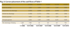
Figure 2 shows correct placement of the cash flows of Table 1 and the formulae in Cell B-20 and Cell B-21 are =NPV(B3,B9:F9) and =NPV (B3,B18:F18), respectively. The above clarification is for ordinary annuity, lease payments based on “annuity due” will be represented by Figure 3.

The difference in the two NALs (Net Advantage of Leasing) is worth noting. When lease payments are based on ordinary annuity, the “lease option” is preferred, but the decision switches in favor of the “buy option” if the lease payments are based on annuity due. This shows that placement of the cash flows (to correctly represent the actual situation) is very critical.
Debt and lease as substitute
This is another debatable issue, which is beyond the scope of this article. For the purpose of this article it is taken for granted that leasing is a substitute for debt financing (as presented in financial textbooks and literature). By virtue of this notion, the analyses assume 100 percent debt for the “buy option.” Therefore, the after-tax or before-tax cost of debt is used to calculate the NPV of each option.
Table 1 shows the loan schedule for 100 percent financing of the asset purchase price of 40,000 using the 10 percent cost of debt. These calculations, however, are not needed as explained below. Most analysts do not pay attention to the concepts involved when doing the calculations.
When an investment is 100 percent financed at an interest rate (i) and the same interest rate is then used to discount the debt cash flow (CFD - interest and principal payments), it results in the same asset value that is used for obtaining the CFD. Therefore, showing the interest and principal payments in such analysis is unnecessary and will reflect the analysts’ lack of adequate command over the subject matter.

Table 2 duplicates the information of Table 1, but instead of the interest and principal payments it uses the asset value at “time zero.” The net advantage of leasing ($1,352) in Table 2 is the same as that obtained in Table 1, but with fewer calculations. The formulae in Cell B18 and Cell B19 are =NPV(B3,C9:G9) and =NPV(B3,C16:G16)+B16 to calculate the NPV of leasing and buy option, respectively.
After-tax and before-tax cost of debt
The above analyses are based on the after-tax cash flow and after-tax cost of debt. Discounting the before-tax cash flow by before-tax cost of debt and the after-tax cash flow by after-tax cost of debt will result in the same value for the NAL. This however, does not mean that the before-tax cash will not include taxes at all. Similarly, the conventional interest calculated based on the asset value (as shown in Table 1) will not work either. The interest deduction in this case is based on the amortization of the equivalent loan. Equivalent loan value is the present value of the cost of leasing as shown in Table 3.

The outstanding balance in Cell-C30 is calculated using =B30-C29-$B4*C28. The same cell is copied to Cells D to G. The rest of the calculations are shown in Table 4. As expected, the NAL = 1,352 is the same as calculated in Tables 1 and 2. The interest tax saving in Table 4 is the interest calculated in Table 3 times the tax rate. Since the after-tax calculations are simpler, those are preferred.
Interest during construction period
The construction period is another area where consistency needs to be maintained and reflect reality as much as possible. As shown in Figure 4, interest during the construction period of a project can be calculated based on three different assumptions. In larger projects, higher interest rate and higher debt/equity ratio situations, the difference could be hundreds of millions of dollars. Using an assumption that does not represent the real situation of debt structure and timing could lead to accepting a bad project/investment.
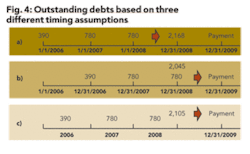
Figure 4 shows the construction schedule of a $3.25 billion project with a debt/equity ratio of 60 percent and six percent cost of debt. As shown in Figure 4, the total debt by the end of the construction period ranges from $2,045 to $2,168 million or a difference of six percent ($123 million). This amount will be used to calculate the debt repayment schedule. To avoid such dramatic differences, the mid-year scenario is recommended for discounting and compounding. Mid-year discounting/compounding assumes that funds are received or disbursed in mid-year. The mid-year compounding or discounting more closely reflects the actual transactions in the treasury. The following shows how the three scenarios in Figure 4 are calculated.

a. 390(1 + 0.06)3 + 780(1 + 0.06)2
+ 780(1 + 0.06)1 = 2,168 b. 390(1 + 0.06)2 + 780(1 + 0.06)1
+ 780= 2,045
c. 390(1 + 0.06)2.5 + 780(1 + 0.06)1.5
+ 780(1 + 0.06)0.5 = 2,105 $
References
1. Mian, M. A., “Revisiting the Pitfalls and Misuse of WACC,” Oil & Gas Financial Journal, October, 2005.
2. Mian, M. A., Project Economics and Decision Analysis - Vol. I: Deterministic Models, PennWell Publishing, 2002.
About the Author

M. A. Mian [[email protected]] is an engineering specialist in the Upstream Ventures Department with Saudi Aramco in Dhahran, Saudi Arabia. He has more than 25 years’ experience in evaluating multi-billion dollar oil and gas projects. Mian is the author of four books “Petroleum Engineering Handbook for the Practicing Engineer, Vol. I and II” and “Project Economics and Decision Analysis, Vol. I and II,” published by PennWell Books, Tulsa, Okla.