Forecasting crude oil futures

Enhacing oil price prediction efficiency with data-heavy market analysis and knowledge of crude oil dynamics
DMITRY SUROVTSEV, SCHLUMBERGER
WITH THE BIG DATA REVOLUTION permeating all facets of the oil and gas industry, energy commodities traders and hedgers are hoping a variety of data-heavy market analysis techniques will help them make more informed decisions about the direction of oil price movements.
However, it appears that most analysts continue to look to the spot market for a guidance in determining their crude oil pricing forecasts, as they have been doing it for decades. More than 30 years ago, the Cambridge Energy Research Associates book The Future of Oil Prices: The Perils of Prophecy uncovered the timeserving nature in oil price predictions: investment analysts tend to forecast low when the spot market is low, and vice versa. Now, in the era of Big Data, the question is can data-heavy market analysis techniques increase the oil price predictive efficiency?
Following the logic expressed by James Surowiecki in The Wisdom of Crowds, a consensus expectation for oil price is best represented by an exchange-traded futures curve. Because investors, traders and hedgers rely on a variety of signals, futures curves are bound to aggregate the predictions from all available market studies performed both by traditional methods (e.g., fundamental, technical, geopolitical) and by new-fashioned techniques, such as social network sentiment analysis.
In this article, we examine how spot market prices have historically influenced crude oil futures-and some of the data-driven techniques that can be applied to reveal key data insights for recognizing eventual spot-price movements.
A 34-YEAR HISTORY OF FUTURES MARKET CYCLES
On today's market, WTI crude oil futures (ticker symbol CL) can be bought and sold for up to nine years in advance. This is a significant change compared to the first CL contracts that started trading on NYMEX in March 1983 with the farthest delivery only nine months away.
To get a holistic perspective on the market, our study is based on the entire 34-year exchange trading history. Using the Quandl financial data platform we retrieved a massive crude oil futures dataset from the NYMEX energy floor inception to date, which, as of June 9, 2017, encompassed 482 individual CL contracts and 8,593 trading days. By organizing the data in the R programming environment, we proceeded to charting the CL futures curves at any desired trading day in the past.
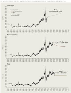
Figure 1 shows three curve shapes observed at random dates: contango (whereby later delivery months are priced higher than prompt ones), backwardation (an opposite of contango) and flat.
An animated visualization of the evolution of daily CL futures curves over the entire 34-year history is available at https://sites.google.com/site/collectivewisdomdatacube/. It is combined with a horizontal gauge displaying the classification of a rolling 200 days' ensemble of curves into the three aforementioned shapes and their relevant bias strengths. The animation also includes a bar chart showing eventual spot price change 3, 12, and 36 months from each trading day.
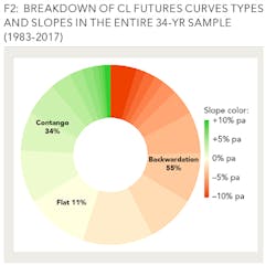
Looking at the curve type breakdown for the entire dataset (Figure 2) it can be observed that the crude oil market is normally in backwardation (which occurred in 55% of trading days vs. 34% of days in contango). For the purposes of this analysis, backwardation is defined as a futures curve slope less than -0.5% p.a. whereas contango features the slopes in excess of +0.5% p.a. The remaining curve types are classified as flat and describe 11% of the patterns identified. Whether these statistics can serve as an argument in the academic dispute on Keynesian normal backwardation theory is outside the scope of the present analysis.
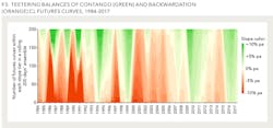
As is the case for any economic phenomenon, it is not surprising that a backwardation market cyclically alternates with a contango one more or less every 2 ½ years (see Figure 3).
FUTURES PRICING DEPENDENCY
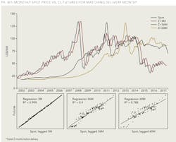
To test the above-mentioned timeserving prediction inference, Figure 4 plots WTI monthly average spot price vs. CL futures for matching delivery months traded exactly 3, 36, and 60 months before delivery. Exactly is a key word in this context since the lifespan of recent CL contracts approached 2,300 business days from the start until the end of trading. Also, shown in Figure 4 are linear correlations between futures prices and lagged spot prices. As can be expected, the farther the prediction horizon, the less dependent is the prediction on the spot price at the time of the forecast. Nevertheless, the latter remained a key determinant (78% importance) even for five-year look-aheads.
FUTURES MARKET PREDICTIVE EFFICIENCY
Having reviewed how spot market shapes price expectations, we now consider if the expectations can influence eventual spot price movements. For this example, we will focus on a 36-month time window.
In doing so we employ a simple Bayesian approach such as used in modern petroleum exploration. Geoscientists know well that a direct hydrocarbon indicator (DHI), for example a bright spot anomaly on seismic lines, does not guarantee prospect success. It increases their ability to distinguish between good and poor prospects. However, a full resolution of exploration risk will only occur after obtaining the results of an exploration well (for conventional resources) or even later, after completing a pilot project (for unconventional projects).
The change in the prospect chance of success (the hypothesis) given evidence (a DHI) can be found using Bayes theorem:
Where H is the hypothesis, E is the evidence, P(H) is the prior probability of hypothesis, P(E) is the probability of evidence, P(E|H) is the probability of evidence given hypothesis, and P(H|E) is the posterior probability of hypothesis given evidence.
Applying the Bayesian framework to the present study, we define the hypothesis as "a spot crude oil price increase by more than 12.5% in three years from a given trading day." In the 30-year data sample, the hypothesis materialized in 3,636 out of 7,435 analyzed trading days, meaning a P(H) of 49%, or a nearly perfect "coin toss" situation.
Playing back the futures history animation, we observed that sharp spot price swings often occurred shortly after the dominant color on the horizontal gauge swiftly changed from red to green (or vice versa). To capture that, we defined the variable B-fraction as "a fraction of CL daily futures curves in backwardation in a rolling 200 days' ensemble ending on a given trading day, in percent" and the variable ΔB-fraction as "a change in B-fraction from 200 days earlier, in percentage points." The evidence is defined as a specific combination of Bfraction and ΔB-fraction on a given trading day.
A valid range for B-fraction is from 0% to 100%, whereas ΔB-fraction can vary from -100pp to +100pp. However, not all combinations of the two variables are possible. If B-fraction is 0%, ΔBfraction cannot be positive. If the B-fraction is 100%, the ΔB-fraction cannot be negative. If the B-fraction is 50%, the ΔB-fraction can only lie in the -50pp...+50pp range, etc.
The full price data sample is represented by the 3D data cube in Figure 5, which features Bfraction on the x-axis, ΔB-fraction on the y-axis, and the log rate of change for spot price on the z-axis. The data point color relates to a price comparison date, that is the date 36 months after a given trading day.
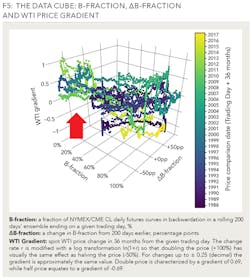
The shape of the 3D figure in Figure 5 appears to confirm the potential of selected predictors to send probabilistic signals for eventual spot price behavior. Note the corner with low B-fraction and low ΔB-fraction that contains very few data points with negative spot price changes (emphasized with a red arrow).
The last step is to create features from the data cube by binning all Bfraction and ΔB-fraction combinations in hexagons. We are now able to assess the Bayesian probabilities of spot oil price increasing by more than 12.5% in three years (see Figure 6).
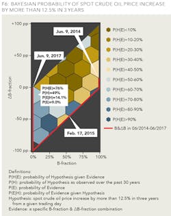
The thick red line at the boundaries of the large tetragon shows the path of evidence movement over the past three years immediately preceding the latest available trading day as of the time of writing (June 9, 2017). These are data points with available x- and y-axis readings but a not-yet-existing z-axis measurement of the data cube. For example, the topmost point on the red line's right edge corresponds to the market situation as of June 9, 2014. The P(H|E) reading of the underlying dark beige hexagon is 39%, which corresponds to "probably not" in Sherman Kent's Words of Estimative Probability. It agrees with the eventual halving of oil price to early summer 2017.
It is encouraging to see that the current evidence position falls inside the blue hexagon featuring a probability of 76% that spot oil price at the early summer of 2020 will exceed today's levels by at least 12.5%.
We stress that the conducted study should not be construed as a new form of technical analysis. It relies on movements in crude oil futures curves to assess the probability of eventual spot price changes. In turn, the futures price curve represents market participants' consensus reached with all presently available market analysis instruments.
The interactive versions of Figures 5 and 6 are available at https://sites.google.com/site/collectivewisdomdatacube/.
WORDS OF CAUTION
To close, a few words of caution are appropriate:
- A probability of an event of 76% does not mean that the event is sure to happen. Borrowing a phrase attributed to the Nobel prizewinner Ronald Coase, "If you torture data long enough, it will confess to anything."
- While CL is the world's most actively traded commodity, over 95% of volume accrue to the nearest 12 delivery months. The exchange settlement prices for farther deliveries are often theoretical.
- Referring to Figure 6, the next evidence movement from the current position can only be in the northeast to east direction since B-fraction can only increase from the current value of nil. That would bring the market state to the light brown hexagon with a probability of subsequent spot price increase of just 26%.
Disclaimer: The views expressed in this article are those of the author and should not be attributed to Schlumberger
ABOUT THE AUTHOR

Dmitry Surovtsev is GeoX Business Manager at Schlumberger. Previously, he worked for Eni, CIFAL, Effective Energy, and Geoknowledge in Kazakhstan, Russia, and Norway. His research interests include exploration and appraisal economics, risk quantification, integrated petroleum-assets modeling, and decision support. He holds an MSc degree in economics from Moscow State Institute of International Relations and a post-graduate diploma in banking and finance from the London School of Economics and Political Sciences.