Newbuild and replacement cost functions

This is part two in a two-part series. Part one ran in the July issue of OGFJ
Mark J. Kaiser and Brian F. Snyder, Center for Energy Studies, Louisiana State University, Baton Rouge, La.
OVERVIEW: Newbuild and replacement cost functions provide insight into the factors that influence costs and are used by investors, companies, government agencies, and other stakeholders to evaluate newbuild programs or the value of an existing rig or fleet. In Part 2, multi-factor cost models for jackups and semis are derived. Water depth was the single best predictor of rig cost and replacement cost models explained larger proportions of variance than newbuild models which is likely due to the manner in which cost estimates were performed.
Newbuild cost models
Single variable models
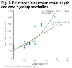
Single variable linear regression models using water depth, year of delivery and drilling depth capability were examined. The relationships behaved as expected in most cases with increases in water depth, drilling depth and build year having a positive influence on cost, however, most relations were not significant. The only statistically significant relationship involved water depth and jackup costs (Figure 1).
Jackups
Multivariate newbuild cost models were specified using an environmental indicator (HARSH), water depth (WD, ft), and water depth squared terms. Variables for country of build, drill depth or delivery year did not add explanatory power and were excluded. The impact of variable deck load was minor and was not included in the best model. The best model took the form:
Newbuild Cost = α0 + α1HARSH + α2WD + α3(WD)2
All costs are reported in million 2009 dollars and the results of several variable combinations are shown in Table 1. Model A explained the largest portion of the variation in newbuild costs and contains both water depth and water depth squared terms of opposite signs. Figure 2 illustrates the output of model A, where the upper line is the model for harsh environment rigs, and the lower line is the model for moderate environment rigs. Costs increase at an increasing rate with water depth, consistent with our prior expectations.

Models B and C compare the effects of the water depth and water depth squared terms and suggest that water depth squared is a slightly better predictor than water depth. In models A through C, negative and large positive intercepts are inconsistent with a priori expectations. Therefore, we examined the effects of constraining the y-intercept to zero in models D through F. The standard error of the regression models through the origin is higher than the analogous standard regression model, suggesting weaker fit. When the y-intercept is set to zero, the magnitude of the coefficients changes, but the signs of the coefficients do not change, suggesting that the direction of the relationships between water depth and operating environments and costs are robust.
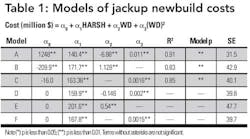
All of the models in Table 1 contain indicator variables for environmental conditions and the coefficients for these variables range from 140 to 201.6 suggesting that harsh-environment rigs are approximately $140 to $200 million more expensive than non-harsh environment rigs which is consistent with the summary statistics described in Part 1 (July OGFJ, pgs. 26-31).
The absence of nation of build and drilling depth variables from the models is not surprising. The lack of a geographic difference is likely due to international competition which forces shipyards to offer competitive pricing. Drilling depth was not a good predictor of costs because it is relatively invariant in the sample with most rigs capable of drilling either 30,000 or 35,000 ft wells.
Semisubmersibles
Semisubmersible newbuild cost models did not yield robust models. The best model of construction costs contained water depth and delivery year:

Newbuild Cost = α0 + α1WD + α2YEAR
The model results are shown in Table 2 with and without the fixed cost component. Both models had similar coefficients but poor predictive ability. The model suggests that for each 1,000 foot increase in water depth capability, cost increases by $25 million, and as the year of delivery increases, costs increase by $38 million. Thus, a semi for delivery in 2012 should cost approximately $100 million more than an identical semi delivered in 2009 because of the market conditions which influence contract negotiations.
For an average 8,333 ft water depth semi delivered in 2010, model B estimates cost at $535 million. Approximately 37% of the cost is associated with the water depth term and 63% is associated with the delivery year term. The influence of the delivery year on costs is time dependent and related to commodity prices and shipyard demand when the contracts were written. Hence, these terms generally do not extrapolate outside the period of analysis and are generally not preferred in the specification. Market conditions in the 2009-2012 period led to increasing price with time; however, if a different time period were selected, conditions are likely to be different. For example, the Sevan Brasil will be delivered in 2012 at a cost of $685 million, but two identical rigs built at the same shipyard for delivery in 2014 each cost $526 million. Understanding the time dimensions of cost is an important determinant of applying empirical relations outside their sample window.
Drillships
No combination of variables was able to capture the distinguishing features of drillship construction. The vast majority of drillships are under construction in Korea which eliminates the country of build variability inherent in the jackup and semi data sets, and orders in the sample occurred over a short time period (2007 to mid-2008) reducing the temporal difference due to market conditions. Additionally, many of the vessels under build are one of three similar designs. In this case, the average cost of drillships adequately describes the characteristics of the sample.
Design Class
Design class was investigated as an explanatory variable for each rig class using the single-factor model:
Newbuild Cost = α0 + α1DESIGN
For semisubmersibles and drillships, design class did not improve the model results, but for jackups, the variable was statistically significant (Table 3).
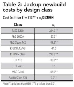
Nine design classes were employed to categorize the sample data and each design class used its own indicator variable such that the cost is equal to the intercept plus the coefficient associated with the design class. For example, to determine the newbuild cost of an F&G Super M2 from Table 3, take the intercept and add -41.6. In cases where the p value of a parameter is not less than 0.05, the parameter cannot be said to differ from zero and the estimated cost is simply the intercept.
The model predicted over 95% of the variance in costs and suggests that there is more variation between rig classes than within rig classes; however, the model cannot be generalized beyond the rig classes depicted. The Letourneau Super 116, the F&G Super M2 and the MSC CJ46 are priced at a discount; the KFELS ModVB, Letourneau 240C and Pacific Class 375 may be considered average; and the KFELS N Class, MSC CJ70 and F&G 2000A are priced at a premium. All three premium designs are for harsh environments.
Replacement cost models
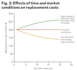
Replacement costs reflect the costs to replace a rig with a new asset of like quality and are related to newbuild cost. For a recently built rig, replacement cost may be estimated by reference to the rig’s original newbuild cost adjusted for market conditions, or the newbuild cost of similar rigs under construction. Replacement cost depends on technology trends, labor and material cost, construction supply and demand conditions, and the age of the rig at the time of the assessment. If new technology and improved construction methods, high competition among shipyards, and low demand for steel prevail in the future, replacement costs will be lower. Conversely, when there is high demand for shipbuilding services and a high price environment, replacement costs increase (Figure 3). Since many of the factors that influence newbuild prices also impact replacement costs, we expect that model results will be broadly similar.
Single variable models
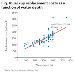
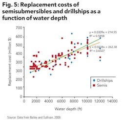
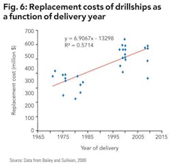
Single variable linear regression models were created to investigate factor impacts on replacement costs. Water depth was a significant factor for jackups (Figure 4) and for floaters (Figure 5). Delivery year was a useful descriptor for drillships (Figure 6) but not for jackups and semisubmersibles due in part to the effect of upgrading which subverts the age variation. Drill depth was not a significant factor for any rig type.
Jackups
Multivariate replacement cost models were specified using water depth (WD, ft), environmental indicator (HARSH), and year of delivery (YEAR, yr):
Replacement Cost = α0 + α1WD + α2(WD)2 + α3HARSH + α4YEAR
Model results are shown in Table 4. Upgrade status was not a useful indicator of costs and was excluded. Age and water depth were significant predictors in several models, but are absent from the best model (model A). Water depth squared was a better predictor than water depth, consistent with the newbuild model relations. Costs increase with increasing water depth, harsh environments, and for younger rigs, as expected. Constraining the intercept to zero had little impact on parameter estimates.
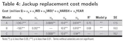
As in jackup newbuild models, the jackup replacement cost model included an environmental indicator with a coefficient of 10.6. This suggests that in the replacement cost sample, a harsh environment rig enjoys a premium approximately $11 million more than a non-harsh rig, much less than for newbuilds and likely due to the capabilities of the harsh environment rigs currently under build. The MSC CJ70 is capable of operating in harsh environments in water depths up to 492 ft, and can drill wells up to 40,000 ft deep with a 7,000 ton VDL; the KFELS N Class has similar capabilities. These additional advanced capabilities make modern harsh environment rigs more expensive than those of the legacy fleet.
Assuming an average moderate environment jackup with a water depth capability of 293 ft delivered in 1982, the replacement cost is estimated by model C to be $131 million. Approximately 60% of the costs are associated with the delivery year term and 40% is associated with the water depth term.
Semisubmersibles
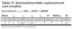
Replacement cost models were specified using water depth (WD, ft), year of delivery (YEAR, yr), and an environmental indicator (HARSH):
Replacement Cost = α0 + α1WD + α2YEAR + α3HARSH
Model results are shown in Table 5. All coefficients were consistent with expectations. The coefficient of the water depth term was 0.020 indicating that for every 1,000 foot increase in water depth, costs increase by $20 million. Newer rigs had higher replacement costs than older rigs, and each year increased cost by $2.2 million. Harsh environment rigs cost $23.8 million more than moderate environment rigs. For the average semi in the sample, model B estimates that 30% of costs were associated with the water depth term and 70% were associated with the delivery year term.
Drillships
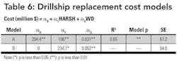
Replacement cost models were specified using an environmental indicator (HARSH) and water depth (WD, ft) variables:
Replacement Cost = α0 + α1HARSH + α2WD
Year of delivery was correlated with water depth and excluded from the model. Results are shown in Table 6. The coefficient of the water depth term was positive and for every 1,000 ft increase in water depth replacement costs increased by $31 million. The harsh environment coefficient suggests that a harsh environment drillship costs $196 million more than a moderate environment drillship. This is far more than the harsh environment premium in the jackup or semi cost models, and is partially the result of semis and jackups being more amenable to modification for harsh environments.
Application
Model application is straightforward. To determine the cost of a newbuild 350 foot water depth, harsh environment jack-up with a 3,000 ton variable load in 2009-2010, for example, we apply the results from Table 1 and select model A since it has a low standard deviation and coefficients with the expected signs. To determine cost we substitute WD =350, VDL = 3000 and HARSH = 1 into:
Newbuild Cost = 1248 + 140*HARSH – 6.88*WD + 0.011*(WD)2
to obtain $328 million. Confidence intervals are calculated using the standard error; a 95% confidence interval is given by $265 to $391 million.
Limitations
The models developed are primarily limited by the sample size of the data from which they are constructed, and for the replacement cost, the manner in which costs are estimated. All three of the newbuild cost models and the drillship replacement cost model had sample sizes under 40 rigs. This is due to the limited drillship fleet size and the small number of rigs under construction at the time of analysis.
Some of the explanatory variables may be subject to error. The models treat the environmental design conditions as a simple variable that can only take the form harsh or non-harsh. However, for jackup rigs, the environmental conditions which a rig can withstand depend in part on the water depth at that location. For example, a rig designed to operate in 350 ft in the Gulf of Mexico may only be able to operate in 200 feet in the North Sea. Overall, water depth was the single best predictor of rig cost. Water depth is believed to serve as a proxy for structural weight, and if weight were included the model fits may improve.
The data provide a snapshot of market conditions at a specific period of time. By fixing the time of assessment the effects of market fluctuations on cost data are eliminated which allows for a better analysis of the physical factors (water depth, harsh environment capacity, etc.) that influence costs. While we suspect that the factors identified as influencing costs apply to the market generally, the value of individual coefficients and model output will change with changes in shipyard supply and demand.
It is possible to build dynamic models of rig cost, but these require a different dataset and model structure, and most importantly, prognostication of market conditions. By constraining the data to a particular point in time, problems with autocorrelation were avoided. While a time-series analysis of newbuild or replacement costs would be valuable, the focus of this analysis was primarily on the physical factors that impact costs. Time-series models may be adequate predictors of newbuild costs, but their application requires the estimation of market conditions in a future period, and given the volatility of the offshore markets, this may prove difficult.
Reference
Bailey, J.E. and C.W. Sullivan. 2009-2012. Offshore Drilling Monthly. Houston, TX: Jefferies and Company.
About the authors
Mark Kaiser is a professor and director of research and development at the Center for Energy Studies at LSU. His primary research interests are related to cost analysis and financial modeling in the oil and gas industry. He holds a PhD in industrial engineering and operations research from Purdue University. Brian Snyder is a research associate at the Center for Energy Studies. His research interests include offshore wind energy and the ecological impacts of energy production.