A modern approach to build 3D sequence stratigraphic framework

Farrukh Qayyum
dGB Earth Sciences
Enschede, Netherlands
Nanne Hemstra
dGB Earth Sciences
Rio de Janeiro
Raman Singh
dGB Earth Sciences
Mumbai
The conventional approach of performing sequence stratigraphy on 3D seismic data is comprised of a limited set of seismic horizons. This practice can be changed with the help of a semiautomated solution that maps all stratigraphically consistent seismic reflectors in 3D.
Modern computer-aided semiautomated workflows are changing these trends. One such approach is utilized in this article. The approach is applied in gas-bearing Pliocene deltaic sands of the Netherlands North Sea.
Using the data-driven approach, three third-order stratigraphic sequences are identified and further classified into systems tracts. The subdivision is performed by integrating the seismic results with the available well data and also by covisualizing the structural and Wheeler (chronostratigraphic) domains in 3D.
This article also introduces several new ideas that add further value to understand sequence stratigraphy. It includes: new stratigraphic attributes, statistical curves, data-driven stratal slicing, and integration of Wheeler diagrams with well data. Some of these ideas are also applied on the presented case study.
It is concluded that the studied interval contains two distinct stratigraphic traps. Sand ridges are elongated downslope traps and are under high risk in the study area because of limited gas charge, whereas several detached shoreface sand bodies are favorable plays in the southern North Sea. This study also documents that the utilized method and workflows are applicable to search for shallow gas stratigraphic plays in the adjoining regions.
Introduction
Modern exploration of hydrocarbons is primarily focused on unconventional stratigraphic traps using large 3D seismic datasets.
This is becoming common because exploration for stratigraphic traps is challenging. It requires not only comprehensive knowledge of sequence stratigraphy but also detailed understanding of seismic data. The latter becomes advantageous if seismic data are fully mapped with a semiautomated method and integrated with high resolution datasets.
General practices in hydrocarbon exploration are to construct a sequence stratigraphic framework by mapping a few sets of seismic horizons. This approach only helps establishing low resolution framework to predict stratigraphic traps and characterize hydrocarbon reservoirs. Seismic data generally contain more information and must be exploited effectively.
Modern attempts are to bridge the gaps between technology and geologic model building. So far, several existing solutions, as explained in the following section, are becoming unconventional practices in stratigraphic trap exploration. These solutions not only help in mapping the seismic data but also to build fundamental understanding of seismic geomorphology and sequence stratigraphy.
This article aims to document the implications of one modern approach of building a 3D sequence stratigraphic framework, predicting stratigraphic trap reservoirs. The secondary objective is to put forward new concepts and their applications in seismic sequence stratigraphic interpretation such as: 3D systems tracts or sequences; new stratigraphic attributes derived from densely mapped data; statistical curves that serve as proxies to understand accommodation and sedimentation changes; predicting paleobathymetry changes from a semiautomated method; and integration of semiautomated Wheeler diagrams with well data.
To explain the objectives in details, a case study is performed. The example is taken from the Pliocene wave-dominated delta of the southern North Sea (The Netherlands). The study documents the presence of stratigraphic traps in the forced regressive prograding deltaic lobes. The understanding of the trap configuration and map is the primary goal of the study that is achieved by performing a detailed sequence stratigraphic study. The results are then integrated with other observations such as vertical fluid migration evident on the seismic data to ratify the existence of secondary gas charge to shallow deltaic sands.
Brief history
Modern semiautomated approaches in performing sequence stratigraphy on seismic data are no doubt following the concepts developed in the history of stratigraphy. The progression was perhaps incomplete without the early groundwork of many earth scientists.
The sequence stratigraphic method itself developed with full of concepts during the 20th century. Later on the advancement in the seismic data gave it further momentum. At present, it has become a formal method in search of hydrocarbons. The following section briefly summarizes the evolution of concepts and their applications in modern semiautomated approaches to build a sequence stratigraphic framework.
Theoretical period
Theoretical period of the developments in sequence stratigraphy is as old as the stratigraphy.The historical roots of sequence stratigraphic concepts date to early findings in stratigraphy when Nicolaus Steno (1638-87) proposed the principles of stratigraphy. His concepts were dealt with the relative geologic time. He initiated the thought that geologists date strata by utilizing the principle of superposition. Following this beginning, many scientists (see also Doyle et al., 1994; Koutsoukos, 2005) contributed in the developments of stratigraphy.
The early discussion on stratal geometries (onlaps, downlaps, and toplaps) was initiated by Grabau (1906). He presented a model and explained various stratigraphic lapouts. His work explained that sedimentation could be controlled by shoreline movement (regression and transgression). His illustration was a regressive dolomitic sequence building outward. He also explained that transgression onlaps the underlying regressive system. This is referred to as Grabau's offlap-onlap model (Miall, 2010). He further explained that the erosion of topsets might occur during both periods: transgression and regression. Therefore, the surface that is developed during this time can form an unconformity or a hiatus.
Barrell (1917) suggested that nature vibrates with rhythms, climatic and diastrophic. He initiated the idea of climatically and tectonically controlled sedimentary systems. He illustrated a geologic column to explain the idea that there are more gaps than record. Furthermore, his illustration expressed the concept of composite cycles of climate and tectonics superimposed on each other. Some years later, Schenck and Muller (1941) introduced the notion of chronostratigraphy to describe the problem created by lithostratigraphy (rock unit) for the time-rock units.
This began the debate of time-based units and their order. The concept of stratigraphic sequences was introduced some years later (Krumbein et al., 1949; Sloss et al., 1949). They called an unconformity bounded unit a sequence. Hedberg (1951) clarified Schenck and Muller's work stating that the chronostratigraphic boundaries are always isochronous. Later on Wheeler (1958)—who is considered the father of time-space diagrams—demonstrated these concepts further by preparing a chronostratigraphic chart that showed alternating base level variations and time stratigraphic units. Any chronostratigraphic chart produced by following his method is now commonly acknowledged as a Wheeler diagram. Sloss (1963) took the base level concept further by subdividing the North American transit cycles into stratigraphic sequences—the term that was defined earlier (Sloss et al., 1949). It was the first practical work in interpreting the tectonic cycles as stratigraphic sequences.
Considering the work of Sloss, Wheeler (1964) expanded the base level variations by illustrating theoretical examples of area-time relationships. He explained that the base level is an imaginary but dynamic surface of earth below which sedimentation occurs. His example was a conceptual drawing of depositional shifts, hiatuses (erosional and nondepositional), and facies changes in time and space. It may be noted that during that time the base level pulses within a basin were explained by studying outcrops using the principles of time stratigraphy as defined by Wheeler (1958).
Applied period: 2D seismic data
Following the aforementioned novel ideas in stratigraphic correlations, the exploration group from Exxon Research (Payton 1977) used the seismic data to explain the subsurface sedimentary cycles within a basin. They created subsurface 2D Wheeler (timespace/chronostratigraphic) diagrams from the seismic data. Following their work, a new stratigraphic discipline was introduced—which is nowadays commonly called sequence stratigraphy. They originally defined it as seismic stratigraphy.
The work of Vail (1975) was to understand the depositional rhythms within stratigraphic units (sequence and systems tracts) as a 2D display of space-time relationship. Their work was mainly a manual interpretation and transformation into Wheeler diagrams. It lacked the third dimension in Wheeler diagrams due to limitations in the availability of 3D seismic data.
3D seismic data
The third dimension emerged progressively with the advances in 3D seismic and computer technologies. It took more than two decades to test a 3D solution to densely map a seismic data and perform sequence stratigraphy (Stark et al., 2013; explain the historical developments of creating seismically driven chronostratigraphic charts.). At present, there are several solutions that exist in the industry to create Wheeler diagrams (Nordlund and Griffiths, 1992; Lomask, 2003; Keskes et al., 2004; Stark, 2005; Ligtenberg et al., 2006; Lomask and Guitton, 2007; Lacaze et al., 2011).
In this article, the HorizonCube method is adopted (de Groot et al., 2010). All approaches have in common that they attempt to fully map the seismic data. The mapping helps in establishing a RGT (Relative Geologic Time) scale, which is thereafter used to create a Wheeler domain, which is equivalent to Wheeler diagrams (Qayyum et al., 2012b).
Methodology
To avoid cumbersome mapping of each seismic event in seismic survey, semiautomated methods are used. One such The HorizonCube approach helps create a set of hundreds of seismic events that are chronostratigraphically sorted. It starts with the 3D seismic data that is transformed into a dip-azimuth volume. The dip-azimuth volume is used to autotrack seismic horizons within a given framework, a geologically constrained model with a set of interpreted seismic horizons and faults. The autotracked seismic horizons are then stored into a volume called 'HorizonCube.'
The method not only reveals that the mapped horizons are chronostratigraphically significant but also extracts key geologic elements (e.g. stratigraphic units, depositional trends, base level changes etc.), which are building blocks for constructing a sequence stratigraphic framework. The horizons could be treated as time (chronostratigraphic) events representing a relative geologic time scale of a rock unit based on the principle of superposition—older at the base and younger at the top. With this advantage, the horizons can be used to carry out a 2D/3D Wheeler (chronostratigraphic) transformation (Ligtenberg et al., 2006). Once the data are transformed into a Wheeler domain, it is ready for sequence stratigraphic interpretation and the integration of results with the well data (logs, core, cuttings, etc.).
The following subsections explain each significant value that the HorizonCube adds in interpreting the rhythms of basin fills and depositional cycles to establish a sequence stratigraphic framework.
Stratal terminations
The first important step towards sequence stratigraphic interpretation is to establish geometrical relationships of seismic reflectors and build fundamental understanding of sequence stratigraphy.
Mitchum and Vail (1977) originally defined various types of relationships (lapouts) that serve as a guideline in interpretation. Based on their guidelines, the HorizonCube events can also be used to understand, map, and visualize the stratal terminations both in structural as well as Wheeler domains. There are two types of HorizonCube: continuous and truncated. The continuous HorizonCube contains mapped events that converge and continue within the entire survey with the continuous events never crossing each other. Such a type can be used for modeling purposes. The second type—a truncated HorizonCube—contains events terminating against each other. The latter type is more stratigraphically significant as it defines the stratal termination (as defined by Mitchum and Vail, 1977). Therefore, the truncated HorizonCube type is recommended to construct 3D Wheeler diagrams.
Stratal stacking patterns
To predict depositional shifts within a base level cycle, one needs to understand the stratal stacking patterns not only on a vertical succession (wireline logs) but also on seismic data (Emery and Myers, 1996). Seismic data have an advantage in this regard because they provide three-dimensional geometrical information.
There are three common stratal stacking patterns used to discriminate one sequence stratigraphic unit from another. These are commonly termed as aggradational, progradational, and retrogradational stacking patterns of strata/reflectors. These stacking patterns are further explained by Catuneanu et al., 2011, with a special focus on shoreline dependent and shoreline independent scenarios. Further quantitative interpretational aspects based on stacking patterns and shoreline geometries are previously covered by Henriksen et al., 2009. Conventionally, the stratal stacking patterns are observed on a 2D section even if one is using 3D seismic data. Such interpretation lacks a three-dimensional perspective of base level changes and the corresponding stratal stacking patterns. The method utilized in this article is capable of mapping and interpreting a sequence stratigraphic unit in 3D.
The HorizonCube method allows the interpretation of these patterns simultaneously in a structural as well as Wheeler domain. Using this method, one can easily slide each mapped event up/down interactively on a workstation to interpret the stratal stacking patterns in 3D.
Automated Wheeler transformation
Wheeler transformation forms the heart of sequence stratigraphic interpretation. After densely mapping seismic data, each automated event is stored as a unique number that corresponds to RGT after transformation in a wheeler domain—which is a three-dimensional flattened domain. The flattening is done for each automated event. Note that the RGT could be later on calibrated with the available biostratigraphic information.
After the transformation, seismic data can be visualized in the Wheeler domain. For stratigraphic interpretation, the data are overlain and integrated with systems tracts isochron attributes and well information (e.g. core images). The transformation of several seismic attributes and rock property cubes in Wheeler domain provide another perspective to understand stratigraphic traps. For instance, predicted porosities in Wheeler domain help in understanding the depositional architecture of stratigraphic traps. Obviously, such information should be used after making the porosity corrections (e.g. compaction; fracture porosity).
The routine Wheeler diagrams always contain one less dimension as pointed out by Qayyum et al., 2012a. That work explained that the Wheeler diagrams only represent the distance-time (if 2D) or area-time (if 3D) information. The stratigraphic thickness per stratigraphic unit is not represented. They proposed a simple solution to compute the thickness of a sequence stratigraphic unit as an isochron volume and plot it on top of an event as a color-coded line. This versatile solution is applicable for both cases: outcrops and seismic. This approach extends the existing Wheeler diagrams. The main benefit of overlaying a Wheeler diagram with the thickness is to incorporate the rates at which the accommodation space is created or destroyed by the sediments in conjunction with the base level variations. One may also create compaction correction volumes based on the preserved sedimentary section and calibrate the result with the biostratigraphic information to understand the rate at which the accommodation space has been filled. If the diagrams are prepared using 3D seismic data, the corresponding Wheeler diagrams that represent all four stratal dimensions are called as 4D Wheeler diagram (Qayyum et al., 2012a).
Systems tracts subdivision
Automated approach only helps to accelerate mapping and transformation of seismic data to Wheeler domain. It is still a job of an interpreter to subdivide the seismic data into meaningful sequence stratigraphic surfaces and systems tracts. This is purely a data-driven approach as this requires observations, covisualization, and interpretation prior to any selection of a model (Catuneanu et al., 2009).
With the knowledge of seismic resolution, the data are subdivided into systems tracts that are the subunits of a sequence. Each systems tract has its own characteristic base level signature and defines a certain type of depositional shift, thus playing a key role in understanding a cycle within a sequence stratigraphic framework.
The systems tracts are subdivided by scrolling the HorizonCube events in the Wheeler as well as structural domain. The key elements in systems tracts subdivisions are the identification of sequence stratigraphic surfaces by correlating the HorizonCube with the well data and by establishing the geometrical relationships of the stratal stacking patterns. The advantage of systems tracts subdivision is that it can be stored as a seismic attribute for three-dimensional visualizations of internal geometrical patterns of the seismic data.A further advantage of the HorizonCube based systems tract subdivision is that one may subdivide the major units into minor units (e.g. parasequences, if observed). Such detailed mapping allows the unraveling of a depositional system within a given geologic time period. For such purposes, the systems tracts subdivision is a most valuable step.
Statistical curves
Statistical curves serve a key product for explaining a depositional system within the context of sediment volume and the filling of an accommodation space. Note that several statistical curves can easily be extracted from the mapped sequences or systems tracts (of a particular order of sequence/cycle). The base level curve is a common curve that is automatically constructed using this method and is in accordance with a chosen depositional model (Catuneanu, 2002).
The theoretical base level curve has a value in interpreting depositional cycles. It is also proposed that the thickness related (mean, minimum, and maximum) statistical curves that define the thickness of a preserved unit are vital tools to understanding how the accommodation space has been filled within a geologic time period. It may be noted that such curves are calculated at a particular location of the basin to explain a particular cycle vertically.
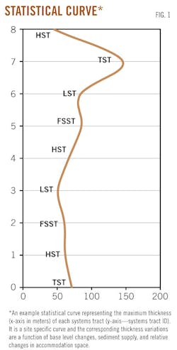
Fig. 1 illustrates the curve of a maximum thickness of systems tracts at a particular location within the survey. The x-axis of the graph represents the thickness in meters whereas the Y-axis represents the unique ID for the units (systems tracts). The graph clearly shows how much an accommodation space could have been filled during a particular base level cycle. Then one needs to integrate the sedimentation response against the imaginary base level curve.
Stratal slicing
Stratal slicing is a method of slicing the seismic data relative to top and base horizons. The idea was first proposed by Zeng et al., 1998. Those authors held that the seismic data are sliced in a model-driven manner to visualize and interpret geomorphologic features.
The model driven in this text refers to proportional horizon slicing that does not honor the data. The advantage of the proposed method is that it is a data-driven approach. Each automated horizon follows the stratal patterns as seen on seismic data. Thus, the method delivers accurate stratal slices to interpret geomorphological patterns. Note that the data-driven slicing through the seismic data reveals depositional changes within an interval, which thereafter could provide insights to the relative changes in base level.
Integration with well data
The densely mapped geometrical information from 3D seismic data can be integrated with the observed log motifs on wireline logs, cores data and with biostratigraphic information. Conventional well-well correlations lack the geometrical information, and thus many pitfalls in interpretation could arise. Seismic data provide such types of information. On top of it, the utilized method helps in mapping, visualizing, and interpreting seismic and well data in 3D. It minimizes pitfalls by providing surfaces that are chronostratigraphically consistent. However, the later step requires calibration of mapped events with the available biostratigraphic information. The underlying concepts and problems in calibrating events with the biostratigraphic data are illustrated in Fig. 2. It is suggested that the calibration should be done within a superposition context by considering a volume of a rock (or rock body) and its corresponding time.
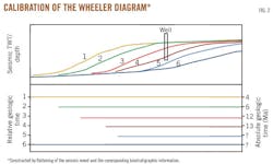
Practical problems arise when one attempts to correlate biostratigraphic/chronostratigraphic ages with RGT scale established with such a method. The common problem is the seismic resolution. Another concern is the economic interest in analyzing a part of a well, i.e. a well drilled within a survey area may not cover the full HorizonCube interval, and it is very common that the biostratigraphic interpretation is not carried out in the entire interval of HorizonCube.
Consequently, not all HorizonCube events can be calibrated in practice. However, one may relate a biostratigraphic marker with a HorizonCube event and assign the corresponding time to the event. After assigning ages, the Y-axis reflecting the biostratigraphic or chronostratigraphic scale may be annotated together with HorizonCube scale. Note that there would be some pros and cons in this approach. The advantage would be that one could calibrate geologic information based on the calibrated scale. The underlying assumption for this practice is that a HorizonCube event is flat; i.e., it corresponds to a rock unit/body time that may or may not be perfectly aligned with a field scale unit. Consequently, the assigned time may represent a gross depositional time for the interpreted unit. Therefore, based on this disadvantage one can still do interpretation at a coarse scale of depositional cycles (of 1st, 2nd, or 3rd orders).
Paleobathymetry prediction
In a preserved stratigraphic record of prograding systems, the height of clinoform geometries can be used as an indicator of water depth. Often, in platform-slope settings, one can use the shelf-slope break point to predict the paleobathymetry developed at that time when the shelf was formed.
This helps in the understanding of depositional settings and the associated environment. It can also be used to calibrate the core/biostratigraphic information with the seismic data or vice versa. If a particular event is a key surface that reflects a predicting paleobathymetry, one can use such an automated event to predict water depth. Note that the paleobathymetry prediction could be difficult in complex geologic settings especially in regions of basin inversion, reactivated fault systems or regions affected by salt tectonism. In such settings, the proposed method would need a special algorithm design and workflow prior to any interpretation.
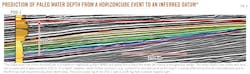
Fig. 3 presents an example of predicting the paleo-water depth between a particular event and a defined datum. The seismically predicted water depth from the datum is 220 m, and the well log (GR) shows a deepening upward trend. The biostratigraphic information of this well suggests marine, sublittoral to open sea connections. Therefore, the predicted water depth from the HorizonCube can be cross validated with the available well information.
Stratigraphic attributes
The geometrical attributes extracted from the densely mapped seismic data are mostly used for stratigraphic interpretation. Four key seismic attributes are directly extracted:
• The HorizonCube density attribute is a measure of number of HorizonCube events within a defined time gate defines. It is done on a trace-to-trace basis. The intervals with higher density values could represent pinchouts, condensed intervals, and unconformities.
• The Event spacing attribute is an isochron thickness between two HorizonCube events. This attribute can also be used to visualize local pinchouts, condensed intervals, and local unconformities.
• The Systems tract attribute is derived from an interpreted HorizonCube. Interpretation here refers to the subdivision of a HorizonCube into sequence stratigraphic units (sequences, systems tracts, or parasequences). Each systems tract can be assigned either a unique or a common number (identifiers). A unique number defines a unique integer value to a systems tract. It is a systems tracts count from top to bottom. A common number defines a common integer value to a systems tract (e.g., highstand systems tract 'HST' = 1). The value remains the same for any further HST interpretation in a volume. Both attributes can be corendered with another attribute to visualize the systems tracts interpretation in a 3D (structural or Wheeler) domain using simple logical expressions as defined by Qayyum et al., 2008. They can also be used as an input for reservoir modeling and characterization as it yields unit identifiers in 3D.
Systems tract isochron is a vertical thickness of a given sequence stratigraphic unit. It is a key attribute to understand how the sedimentation filled the basin over a relative geologic time if it is visualized in a Wheeler domain. Interpretation is done on the HorizonCube itself by integrating the mapped events with well data. The attribute volume can be used to describe depositional shifts, condensed sections, erosional features, etc. It can be used to generate pseudocompaction related volumes that can be used as an input for basin modeling. It can also be used as an input to reservoir modeling.
Note that the above discussed attributes are the physical attributes of strata defined at the seismic scale and thus add value to sequence stratigraphic interpretation in the Wheeler domain. Other geometrical attributes that could yield similar results also exist (Rickett et al., 2008; Lomask et al., 2009; van Hoek et al., 2010).
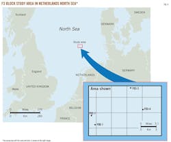
Case study—North Sea
Data set
The seismic dataset used in this case study is located in the F3 Block (Dutch sector) of the southern North Sea (Fig. 4). The data cover 387 sq km. The seismic data were processed up to prestack time migration (PSTM) and a further poststack smoothing filter was applied prior to the HorizonCube preparation. Additionally, four wells containing sonic, density, and gamma-ray logs are used in this study.
Generalized geology
The Pliocene interval of the North Sea is comprised of deltaic cycles ranging from a river-dominated to a wave-tide dominated stages. These cycles are comprised of classic clinoform geometries prograding towards the basin. The interpretation revealed three third-order sequences (wells correlation, Fig. 5). The sequences are developed due to the enlargement of a large-scale fluviodeltaic drainage system (Eridanos delta) that dominated northwestern Europe during the late Cenozoic. The drainage system started during Oligocene while the Scandinavian shield was being uplifted. The uplift rate increased during the late Miocene and again in early Pliocene (Ghazi, 1992; Jordt et al., 1995).
Because of late Miocene uplift, high sediment influx filled the northern offshore regions of the Dutch sector. The increasing sediment load has resulted in a differential load throughout the region. Consequently, the buried Permian Zechstein salt started moving in the region and several localized unconformities were formed within the Pliocene interval that are underlain by salt domes (Fig. 6). Some unconformities with a similar origin are identified in this case study after HorizonCube preparation and subsequent Wheeler transformation (for references, please refer to the earlier work of Qayyum et al., 2012b).
Biostratigraphic information of the northern part of the study area has been earlier done by Kuhlmann et al., 2006. Rest information on relative age(s) are available on the TNO website (www.tno.nl) as are classic biostratigraphic reports of wells (Jansen and Gervais 1997, 1999).
Pliocene depositional cycles
The depositional cycles are first interpreted by correlating the well data using the key wells that form the basin dip orientation (Fig. 5). The correlation is done by following the principles of sequence stratigraphy and the depositional model IV (see Fig. 28 in Catuneanu, 2002). Note that this model suggests four systems tracts within one complete base level cycle. The information obtained from the well data are afterwards integrated with the mapped seismic reflection patterns, i.e. HorizonCube. Based on such correlation, the depositional cycles are subdivided into systems tracts. Further inspection of the 3D nature of the interpreted systems tracts is done by interpreting the 3D Wheeler diagrams, 3D Systems Tracts attribute, and the systems tracts thickness volume. The interpretation of the interval is described below.
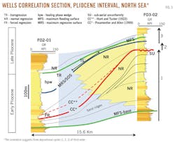
Well correlation
The Pliocene interval is comprised of siliciclastics deltaic units that are prograding basinward. Each unit is very sandy and is often separated by the intercalations of siltstone and marine shales. The wells correlation section (Fig. 5) shows two clear maximum flooding surfaces (MFS)—one at the base of the Pliocene interval (MFSbase) and the other at the top (MFS). Three depositional cycles are interpreted. The basal depositional cycle is mainly a normal regressive systems tract bounded by a distinct MFS and SU (subaerial unconformity and its correlative conformity-CC).
The intermediate cycle-2 is quite complex on this well section, and it is not easy to correlate in the basinward direction. It contains a couple of regressive units that are thin landward and thick basinward. It is interpreted that such a cycle might contain forced regressive (FR) units that are detached from the shelf. Seismic interpretation is unavoidable for this cycle as the well correlation (in this case) certainly requires incorporating geometrical information. The upper
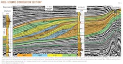
depositional cycle-3 contains a distinct healing phase wedge (transgressive systems tract – TST) sandwiched between normal regressive units. The well correlation shows the prograding cycles (1 and 2)—note the basinward progradation of the coarsening upward succession—that correspond to the river dominated stage of the Eridanos delta during the Early Pliocene stage. Using seismic data, the same wells are correlated to obtain more geologic information (Fig. 6) based on seismic reflection patterns. With the advantage of the HorizonCube, each seismic reflector is interpreted and correlated with the well's motifs (e.g. coarsening/fining upward trends).
The well correlation suggests that there are three depositional cycles that have been deposited within duration of 3.5 Ma. Therefore, the depositional cycles are of 3rd order and the corresponding sequences are referred as 3rd order sequences. The further interpretation of these sequences is done using the HorizonCube in the entire 3D survey area.
Pliocene third order sequences
After correlating the well with seismic data using HorizonCube, the same three cycles are subdivided into sequence stratigraphic units—sequences and systems tracts (Fig. 6). Furthermore, the seismic data are also transformed into a Wheeler domain to simultaneously interpret the data in the structural as well as the stratigraphic domain (Wheeler diagram). Note that if one follows the conventional method of preparing the Wheeler diagrams, the unit thickness is not illustrated. The reason behind this is that the Wheeler diagrams have always been prepared by looking at the lines and their spatial extent in 2D. The thickness of a unit has always been ignored.
Earlier Wheeler and Maurice (1948) criticized this and said that without the scale distortion one cannot illustrate the thickness if the geologic time is considered. They suggested that one should either consider thickness or time to illustrate a stratigraphic unit. However, it is recently proposed (Qayyum et al., 2012a) that one should not ignore the thickness of a unit while interpreting the Wheeler diagrams. The thickness per systems tract is computed and posted as an overlay in the Wheeler domain (Fig. 7). In this manner, the depositional cycles of the studied interval are interpreted not only to look at the depositional trends but also interpret how the accommodation space has been filled over the relative geologic time. The interpretation of the sequences and the systems tracts is given below.
The lower cycle-1 is interpreted as sequence-1 that is comprised of TST, HST (highstand systems tract), and FSST (falling stage systems tract) within the early Pliocene interval. The basal unit (i.e. TST) of this sequence is landward restricted (Fig. 7). It contains chiefly sand ridges that are overlain by thin transgressive shale (e.g. GR log of Fig. 5 of the wells correlation). It is overlain by aggrading to prograding parasequences sets. These sets collectively form a HST. The HST prograding events downlaps onto the earlier defined MFS of TST. Following the HST of sequence-1, the base level fell during the early Pliocene stage. The work of Westaway (2002) suggests a regional uplift in the entire region during the Pliocene-Pleistocene stages. This mainly suggests a thick-skinned tectonic phenomenon. However, considering the scale of the F3 survey and the underlying Zechstein salt that has intruded into the overlying sediments, it is interpreted that the salt tectonics has also played a role. The eastern part of the survey is underlain by two domal structures—containing salt in the core. Just above these domal structures, the topsets of the HST are eroded. Therefore, the fall in base level is a controlled by thin as well as thick-skinned tectonics. The top of HST is interpreted as a subaerial unconformity (SU). The corresponding falling stage unit is formed in the basinward direction (see Wheeler diagram of Fig. 7) that shows a detached forced regressive unit. This falling stage is interpreted as a falling stage systems tract (FSST). On the wells correlation (Fig. 5), this unit (FSST) cannot be clearly identified and its geometries are better understood on the seismic data. The top of FSST is interpreted as a correlative conformity 'CC**' (Hunt and Tucker 1992), and its base is interpreted as a basal surface of forced regression (BSFR).
The overlying stratal stacking patterns in structural as well as in Wheeler domain form an aggrading to prograding unit (Fig. 7). The entire succession is mainly coarsening upward parasequences set on the well section and it forms a thinly defined equivalent unit in the basinward direction (Fig. 5). The unit is mainly a normal regressive (NR) systems tract.
Considering one sinusoidal base level cycle of four systems tracts (TST, HST, FSST, LST), this unit overlies the previously defined TST and it is more proximally located. Therefore, this unit is interpreted as a HST. The stage is a mature deltaic cycle that appears to pass the previous shoreface and underlying sand ridges due to high sedimentation rates and larger accommodation space. Therefore the rate at which the accommodation space is being filled is more than the rate at which the base level rises at the shoreface. Note that there are some sequence stratigraphic surfaces (e.g. basal surface of forced regression— BSFR, correlative conformities 'CC' forming, top of forced regressions, and SOS—Slope onlap surface) that cannot be interpreted easily based on wireline logs and such surfaces are purely geometrically defined. According to Embry (2009), correlative conformities are time based surfaces. Most of these surfaces appear quite clearly in the study area and are automatically mapped correctly based on the dip/azimuth information. The 3D mapping suggests that the topsets are eroded over a larger area (covering 110 sq km) within the survey. The basinward extension of the paleo-seafloor during the highstand stage is the BSFR. The term paleo-seafloor for this surface was originally defined by Posamentier and Allen (1999). According to them the surface forms a correlative conformity 'CC*' while the highstand delta progrades basinward.
The intermediate cycle-2 is interpreted as a sequence-2, which was not clear on the dip-oriented well correlation section (Fig. 5). It is comprised of chiefly regressive units (LST, HST, and FSST). The lowstand systems tract (LST) that overlies the FSST of sequence-1 is located in the basinward direction and it shows a rise in base level after the earlier fall in base level. The LST contains marginally prograding units in the F3 block. There is another normal regressive unit interpreted above the LST of sequence-2. The unit mainly shows aggradation in the coastal plain settings (previous topsets of HST of sequence-1) and progradation in the basinward direction. The unit is interpreted as a HST of sequence-2. On seismic, a distinct incised valley is also observable, which suggest a relative fall in base level at the coastal to shelf setting (Qayyum, 2008). It is interpreted as a second falling stage of the Pliocene cycle and the corresponding unit is termed as FSST. This completes the second cycle of deposition, and the top of this cycle is interpreted as another sequence boundary—which is a composite surface of SU and CC. Note that this sequence-2 does not contain any interpreted TST within the base level cycle-2 because it was not fully resolved at seismic scale. It is interpreted that the TST is very thin and cannot be identified at the seismic resolution of this data.
The last cycle-3 is mainly a stage when the basin starts rising after the fall stage of cycle-2. The corresponding regressive unit is interpreted as LST that is again basinward restricted and shows prograding patterns. After the deposition of LST the base level rises and a marine onlap forms in the slope setting defined by the LST slope. During this stage, the rate of rise in base level is faster than the rate at which the sediments are being brought into the basin. Therefore, a distinct healing phase wedge is formed. It also shows a clear MFS that could contain transgressive lag deposits (Fig. 5). The wedge is overlain by a normal regressive systems tract, i.e. HST. This cycle-3 is interpreted as sequence-3 that corresponds to the late Pliocene age.
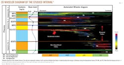
3D Wheeler diagrams
The 3D HorizonCube of the studied interval has also allowed for the preparing of a 3D Wheeler diagram of the Pliocene interval of the southern North Sea in the F3 Block. In Fig. 5, the vertical sections are the Wheeler transformed seismic sections, and the horizontal slice is the lowermost
MFS of the sequence-1. Note that the 3D Wheeler diagram clearly shows the transgressive, normal regressive, and forced regressive sequences. All three sequences are now evident in 3D. The diagram shows a large time gap between the sequence-1 and sequence-2 in the NE direction. This is interpreted as a hiatus within the Pliocene interval. The top of this hiatus is interpreted as an unconformable surface or a sequence boundary (SU+CC)—for details see Fig. 6. Its geometry and areal extent has also been interpreted by using the HorizonCube density attribute as is explained in the seismic geomorphology subsection of this article.
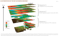
3D systems tracts
The interpreted third order sequences and the corresponding systems tracts are also visualized in 3D (Fig. 9). Note that each systems tract has its own spatiotemporal framework. With thickness attribute as a volume, each systems tract represents its own four dimensions. Such a visualization that contains all four information is here referred as 3D systems tracts. The visualization is further extended by displaying a set of key events in Wheeler domain (Fig. 10). Both figures bring the 3D nature of a stratigraphic unit within the study area and highlight the depositional shifts clearly.
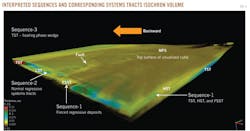
The depocenters or the thicker locations of a systems tract are evident within the survey area. It illustrates that the sequence-1 and sequence-2 are closer towards east and quite thick prograding systems. However, the sequence-3 is distally located and thinner than the earlier one. The Wheeler diagram (Fig. 8) also shows the spatial extent of forced regressive (FR) unit with an unconformity (where horizon slice is stopping). Also note how the thicker regions move their areas over the RGTs.
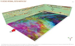
Seismic geomorphology
The benefit of having the HorizonCube in this case study was that it was not only used to analyze seismic attributes along the events but it has also delivered new geometrical attributes (e.g. read the section in this text). The mapped events are used to understand two key geomorphological aspects of the Pliocene interval: sand ridges in the sequence-1 and the SU attribute volume in conjunction with paleo-seafloor of sequence-1 (Fig. 6). Sand ridges of the TST (sequence-1) are studied with the aid of the HorizonCube and seismic attributes along the events. The ridges form elongated NNW-SSE to NW-SE trends (Fig. 8). Further inspection of seismic attributes (spectral decomposition) suggests that these elongated features are analogous to the present day offshore sediment transport (longshore drift) in the Dutch Sector—see Fig. 1 in Walgreen et al., 2002. The longshore drift has formed the elongated sand ridges perpendicular to the present day coast of the Dutch Sector. With the passage of time, the Dutch coast is being modified due to a rise in base level (marine transgression) and several tidal inlets and barrier islands are formed. This suggests an intermediate stage of tide to wave dominated deltaic settings—in which the tidal and wave action is dominant over the river power. Note that such settings could also form barrier islands near the previous coast and offshore the sediments are being deposited due to superimposed sedimentary processes. The most common sedimentation phenomena are the longshore drifts, sand storms, and tidal action for the sand transport. Walgreen et al. (2002) have taken the present-day observations of the Dutch coast a step further by proposing a model based on morphology based basin dynamics and sand transport. Their model suggests that the shoreface-connected sand ridges could be formed during the storm conditions. Such a case has also been observed in the early Pliocene interval of the F3 Block with an average height range of 10-20 m.
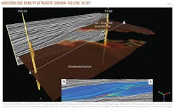
The second morphology is extracted using the density attribute of the intervals defined by SU and BSFR (top of sequence-1). The attribute is visualized in 3D by putting a transparency to the color values that have low density values and visualizing all regions of higher density values (Fig. 11). The result presents a classic region of SU that covers an erosional area of 110 sq km in the landward direction whereas the BSFR forms a condensed area of 190 sq km in the basinward direction. It may be noted that this BSFR represents a paleo-seafloor in the F3 Block. The paleo-seafloor is overlain by the FSST that happened soon after the erosion of HST—as defined by SU.
Implications: North Sea shallow gas exploration
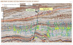
Recent discoveries of shallow gas in Plio-Pleistocene delta of the Netherlands are in the unconsolidated sandstone (e.g., A-15 and adjoining blocks that lie north of the study area—for details see Stuart and Huuse, 2012). These sandstones are filled with gas due to secondary migration of gas due to Zechstein salt tectonics that resulted into a seal failure (Schroot and Schuttenhelm, 2003). The gas moved upward through a major fault plane (Fig. 12), which thereafter charged the overlying regressive sand rich systems tracts.
The F3 Block contains two important sand-prone stratigraphic plays in the Pliocene deltaic system. Sand ridges form the first prolific elongated reservoir bodies that are formed parallel to the Dutch coast (see Sand ridges in Fig. 8). The bodies are being capped by a distinct MFS that fills the adjoining regions of elongated sand ridges with muds and claystone—forming a stratigraphic trap. These traps are available in study area but are under high risk because of limited to no secondary fluid (gas) migration. Nevertheless, these bodies extend from south to north during this period and the prolific sand ridges traps lie above the underlying Zechstein salt domes if the Tertiary systems are not severely faulted. A classic example is the A-15 block that contains the recent discoveries in similar environment.
The forced regressive wedge—referred in this article as FSST of sequence-1—is another stratigraphic play. It forms a significant trap in the study area. These sands are bypassed sedimentary units within the FSST (Fig. 12). These traps are also previous shoreface parallel and elongated traps underlain by a salt dome. There is a distinct seal failure and gas chimney indicative on the data (Fig. 12) that explains the secondary migration, which charges the sands corresponding to this FSST.
Discussion
In most of the interpretation workflows, the static models (which serve as an exploration and development tool) are always coarse and thus detailed information is ignored. The benefit of this method is that one builds a detailed static model. Furthermore, the sequence stratigraphic framework is also built in 3D.
The method is unique, and this article serves as a guideline in interpreting the subsurface based on seismic and well data using a semiautomated method. It delivers a full 3D view of the subsurface that is conventionally not possible despite the fact that a 3D seismic data are acquired. Not only this, it is also proposed that without the well integration automated approaches could be useless. Contrarily, without having a 3D geometrical view, wells correlation could also be limited although the well data have better resolution but lack the spatial resolution. Stand-alone wells correlation is not going to give full information. However, if the mapping has been done using all possible seismic reflections, one could slide them in a geological manner to correlation well motifs and attempt to see why a certain depositional trend is distinct to a well. This gives a start to explain the things logically and thereafter to construct a depositional model with confidence. It is just a start of full integrated 3D sequence stratigraphic interpretation that allows building of a hierarchal (1st, 2nd, and 3rd order) depositional framework.
Conclusions
Detailed sequence stratigraphic framework is only possible if one maps the seismic data completely. This approach helps in establishing a detailed and integrated sequence stratigraphic framework. The case study explains the implications of the adopted approach.
The study identifies three third order depositional sequences within the Pliocene prograding delta. These sequences are predominately within the wave-dominated settings. Nevertheless, the delta itself is a sand-rich system that is a host of potential shallow stratigraphic traps in the region. Amongst those, only two key traps are discussed in the article: sand ridges and FSST. The other prolific known reservoirs in the area are structurally controlled traps and those form the shallow gas pockets. Those form clear and distinct bright spots on the seismic data and thus beyond the scope of this article to be discussed in detail.
This study concludes that modern semiautomated workflow only helps in accelerating the mapping. For successful stratigraphic trap prediction, one still needs to subdivide the seismic data into meaningful sequence stratigraphic units by covisualizing various results and integrating them with the well data in time and space. The dense mapping yields several 3D perspectives that are advantageous to understand the sequence stratigraphy and predict stratigraphic traps.
Acknowledgment
The authors acknowledge the Dutch government for releasing the dataset and TNO for allowing dGB Earth Sciences to publish the data online under creative common license (www.opendtect.org/osr).
References
Please email the first author for a list of full references.
The authors

Farrukh Qayyum ([email protected]) joined dGB as a geoscientist in April 2008. He is involved in sequence stratigraphic interpretations, seismic object detection, and interpretation studies. He also worked for Schlumberger and Baker Hughes Inteq. He holds an MSc in geophysics and an MPhil with specialization in sequence stratigraphy from Quaid-i-Azam University.

Nanne Hemstra is dGB executive vice-president Brazil and a senior geoscientific software engineer. He is a founder of OpendTect and has been involved in almost all OpendTect developments since he started working for dGB in 2001. He holds an MSc in geophysics from Utrecht University.

Raman Singh is a manager of software development at dGB India. He graduated from the Indian Institute of Technology in geoscience in 2003 and worked with Reliance Industries Ltd. in Mumbai before joining the OpendTect development team at dGB in 2007.