Integrated fracture models require space-, time-dependent parameters

A consortium of operators produced simulation models from Delaware basin, Midland basin, and Bakken datasets to determine the effects of proppant distributions, far-field depletion, and long-term proppant degradation on long-term production. Observation wells, cross-well and injection-well fiber, interference tests, post-fracturing perforation imaging, and production data combined to calibrate the models.

Each dataset required key parameters for history matching. These parameters revealed that proppant trapping by fracture roughness determined propped length and height, and formation properties and proppant mesh size directly affected the magnitude of proppant trapping. Realistic estimates of proppant trapping for model simulators are provided from the history matches.

During production, fractures experience large pressure gradients which affect fracture performance as a function of time and distance from the well. Fracture conductivity typically decreases over a 5-year period, with conductivity reduction accelerating after 2 years.

Integrated modeling

Researchers at ConocoPhillips Co., Hess Corp., ExxonMobil Corp., and Apache Corp. used a fully-coupled hydraulic fracturing and reservoir simulator to evaluate long-term production trends in Permian basin and Bakken shale wells. Extensive diagnostic and production data characterized the size and shape of hydraulic fractures in the wells to produce calibrated production models. These models provided insight into near-and far-field fracture and proppant propagation. Long-term production and modeling investigated depletion effects on the fracture networks.

MB1 dataset

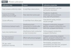
The MB1 dataset included multiple wells targeting the Wolfcamp B formation in Midland basin. Model calibration was done for west pad Wells E, G, and D. Upper Wells E and D were in the Wolfcamp B-1 layer, and lower Well G was in the Wolfcamp B-3 layer. Fig. 1 shows the relative locations of the wells and well spacing.

Multiple well-pairs with cross-well fiber data defined fracture geometries using frac hit data. Frac hits relative to the monitoring well outlined minimum and maximum frac extensions, and in-well fiber observations from neighboring pads determined cluster efficiencies. MB1 had 50-60% cluster efficiency.

Well connectivity was obtained by interference tests conducted at 16-month intervals. These tests also provided proppant conductivity estimates during long-term drawdown. Oil, gas, and water rates for 3.5 years of production provided data for production history matching. Similar interference tests and three-phase production data were collected for the other wells in the study. Table 1 shows the parameters for calibrating the model which were also applicable to the other well datasets in the study.

DB1 dataset

The DB1 dataset consisted of six horizontal wells with three landed in Wolfcamp A and three in Third Bone Springs in Delaware basin. Fig. 2 shows a gun-barrel plot with well locations and spacings. Well completions included stage designs with 100-, 200-, 250-, and 350-ft stage lengths incorporating 4-, 8-, 10-, and 14- clusters/stage, respectively. All stage designs used similar fluid and proppant loading per cluster and surface injection rate/stage. Total number of perforations in a stage were kept constant regardless of number of clusters in a stage, resulting in similar limited entry pressures among the wells.

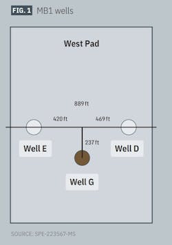
Fluid rate/cluster, therefore, varied among the designs. Fiber data monitored Well 2A in Wolfcamp A and measured frac hits between 880-920 ft in Wolfcamp A and 320-780 ft in Third
Bone Springs. Perforation imaging interpreted fluid and proppant distributions between clusters for the different stage designs.

Production allocation was via spinner logs.

BK1 dataset

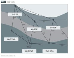
The BK1 dataset consisted of one parent and five child producing wells in the Bakken with an additional monitoring well. Fig. 3 shows a gun-barrel plot with four producing wells in the Middle Bakken and two producing wells and one observation well (H4) in Three Forks. Wells H4 and H5 contained fiber for monitoring. In-well fiber data during the H5 stimulation determined about 100% cluster efficiency.

BK2 dataset

The BK2 dataset consisted of one production well drilled in the Middle Bakken and pressure-monitoring wells in the Middle Bakken and Three Forks directly underneath (Fig. 4). Monitoring wells were cased and cemented but not perforated. They contained cemented fiber and an external casing pressure gauge array to record formation pressure during stimulation and long-term production.

Fiber optic data estimated the distribution of fracture lengths and propagation velocities. The slanted orientation of the Middle Bakken monitoring well provided an estimate of far-field fracture hit efficiency (cluster number/fracture hits).

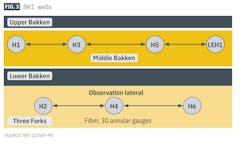
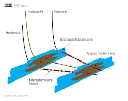
The Three Fork monitoring well measured nearly 100% fracture hit efficiency for all clusters. BK2 had 95-100% cluster efficiency. The monitoring wells each contained 15 pressure gauges spanning both vertical and horizontal distances from the production well.

Pressure measurements represented pressure in the fractures which was communicated to the pressure gauges though conductive paths to the outside of the monitor well laterals. Fig. 4 shows the pressure decrease in the offset gauges during production over time.

Model calibration

Production modelling required an integrated hydraulic fracturing and reservoir simulator. Required parameters for the model include:

Horizontal, vertical fracture toughness measurements.
Vertical stress profile.
Fracture conductivity during propagation, balancing toughness and the viscous pressure drop affecting fracture morphology.
Maximum immobilized proppant (MIP).
Modified Kozeny-Carman coefficient (K0).
Proppant conductivity loss as a function of time.
Reversible pressure-dependent permeability increase during hydraulic fracturing.
System permeability.
Relative permeability curves.
System permeability pressure-dependencies during drawdown.
Fractal dimension parameter to account for variable spacing in fracture swarms.

MIP holds up proppant in the fracture due to fracture roughness, ledges, and small-scale irregularities. MIP is expressed as lb/sq ft of proppant trapped. Forcing proppant to transport vertically due to high MIP limits horizontal reach.

MIP, therefore, provided a key calibration parameter for effective proppant length matching in addition to gravitational settling.

A modified Kozeny-Carman equation calculated proppant pack conductivity, where K₀ replaced the typical 0.0056 coefficient. Singular laboratory K₀ estimates typically do not adequately capture conductivity variations throughout the fracture network, and field data provided better values for K₀ distribution for the models.

Model calibrations included fracture-hit timing and hydraulic half-length constraints. These parameters, in addition to toughness and reversible pressure-dependent permeability, calibrated fracture geometry. An erosion coefficient α, calibrated cluster efficiency.

K₀, time-dependent conductivity loss, proppant embedment, proppant trapping, and proppant
conductivity loss with effective normal stress calibrated fracture interference. Proppant trapping and K₀ calibrated early time interference. This interference was due to high connectivity between the wells at the start of production.

Conversely, proppant conductivity degradation with time and effective normal stress calibrated late-time interference.

Model calibration

The four separate datasets required somewhat different approaches to model calibration, but in general all models used similar key components for history matching. These components included fracture-hit timing, hydraulic half-lengths, cluster efficiency, early and late time interference, proppant embedment, proppant trapping, proppant conductivity loss, and cumulative production.

Fracture toughness guided distance-dependent fracture hits to determine fracture half-lengths.

Horizontal vs. vertical anisotropy determined fracture height. Limited entry-perforation efficiency data combined with perforation tensile strength provided cluster-efficiency calibration.

Early production interference tests calibrated proppant trapping, K₀, and proppant conductivity degradation with time and effective normal stress calibrated late-time interference. Likewise, far-field pressure gauge observations calibrated proppant conductivity parameters. Permeability and relative permeability curves tuned production for history matching.

Calibration results

Results from the four datasets showed that fracture-geometry matching required accurate assessment of the vertical stress profile and the minimum horizontal stress (Shmin) distribution across the layers. These parameters described the fracture network. Proppant transport through the networks, however, depended upon the geological setting, proppant mesh size, and flow rate.

Immobilization proppant values between Bakken and Midland datasets showed how geological properties affected the proppant distributions. BK calibrations required 0.07-0.15 lb/sq ft MIP
whereas the DB calibrations needed 0.1-0.3 lb/sq ft MIB, depending on volumetric flow rate.

he higher trapping values resulted from fracture roughness, natural fractures, and other geological features causing proppant holdup.

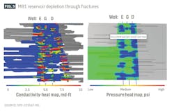
Fig. 5 shows conductivity distribution in the fractures in the MB1 history-matched model. Early-time (6-month) production was primarily controlled by proppant conductivity distribution (left panel). The right panel shows the 5-year far-field pressure depletion profile. Late-time depletion depended on both early- and late-time conductivity distribution, with the latter depending upon an accurate history-matched model.

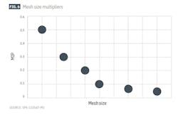
MB1 reservoir depletion through fractures (Fig. 5)

The BK2 dataset revealed the importance of proppant mesh size on conductivity patterns. The BK1 calibration required a single MIP of 0.15 lb/sq ft, but the BK2 dataset calibration required multiplying the baseline 0.07-lb/sq ft MIP by the mesh size through multipliers, decreasing conductivity with distance from the wellbore. This functionality results in coarser proppant immobilized closer to the wellbore, where fracture tortuosity would naturally trap larger particles and finer proppant would be transported further into the fracture network. Fig. 6 shows the mesh-size multipliers used in the BK2 calibration.

DB1 required modeling MIP as a function of flow rate per cluster due to large differences in production between 100-ft and 200-ft stage lengths. This approach assumed that higher velocity more effectively transported proppant further from the wellbore. Fig. 7 shows the fracture network in a 200-ft and 100-ft cluster model. The 100-ft stage design had higher velocities in the near wellbore areas of the fracture network compared with the 200-ft stage design. To account for proppant transport and settling in these different cluster lengths, the history match used 0.3-lb/sq ft MIP for 200-ft stages and 0.1-lb/sq ft MIP for 100-ft stages.

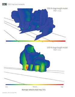
The lower MIP value produced a larger propped area in the cluster which resulted in higher production.

Time-dependent conductivity loss occurs due to proppant crushing, slow embedment, fines migration, inorganic scaling, and accumulation of insoluble organic material. Laboratory measurements do not adequately test these long-term trends. BK2 data could only be history matched using decreasing fracture conductivity as both a function of pressure drawdown and time.

The MB1 model required significant time-dependent conductivity loss to match the rate-transient analysis (RTA) trend. Fig. 8 shows the fracture conductivity profile for the matched MB1 dataset for 6 months, 2 years, and 5 years of production.

The colors are log-scaled from 0.05 to 50 md-ft and show reduced conductivity in the fractures over the 5-year period, with conductivity reduction accelerating after 2 years.

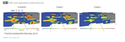
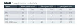
MB1 time-dependent conductivity loss (Fig. 8)

Table 2 summarizes history-matched propped fracture conductivity for the four datasets. High and low values outline conductivity variations as a function of distance from the wellbore and between fractures due to heterogeneity in proppant distribution. For the DB1 dataset, conductivities vary with stage length, and the table reports only the 200-ft stage length values.

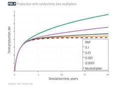
For general preliminary long-term production analysis, it was recommended to use minimum time-dependent conductivity loss multipliers from 0.001 to 0.01 which smoothly and asymptotically approach the final conductivity values.

Higher multipliers result in more production by slowing conductivity degradation over time. Fig. 9 shows the effects of the multipliers on long-term cumulative production.

Production with conductivity loss multipliers (Fig. 9)

The results of the model studies showed that fractures exhibit a large pressure-gradient during long-term production. Fracture conductivity diminishes with distance from the well, with pressure drawdown, and as a direct function of time. Early production experiences high pressure drawdown but declines after the first year when time-dependent conductivity loss begins to dominate.