Machine-learning models predict produced water properties

Produced water composition reveals subsurface structures and provides a basis for scaling tendency prediction. Saudi Aramco developed a machine learning (ML) workflow that classifies produced water to avoid misidentification of water sources which could lead to erroneous reservoir assumptions.

SLB developed a machine-learning-based reduced order model (ROM) to quantify physicochemical properties and scaling tendencies of oilfield waters and replace rigorous, first-principle thermodynamic models. The ROM runs faster and is easier to integrate into digital workflows than first-principle models and provides suitably accurate results.

Water source identification

Subsurface flow analysis using geochemical compositions of oilfield water identifies hydrocarbon migration and reservoir compartmentalization. For example, gradual salinity increases in a formation water system indicate a connected hydraulic system. Similarly, local homogeneous samples among wells indicate a permeable flow pattern and hydraulic connectivity between wells and formation. By contrast, abrupt differences in formation water composition on a local scale suggest the presence of hydraulic barriers and compartmentalized subsurface structures.

Foreign water sources from drilling and completion fluids or water for injection,

however, can mix with formation water, complicating the analysis and potentially leading to erroneous conclusions.

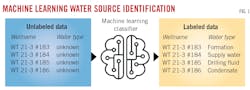
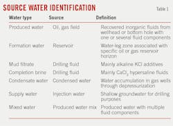
Saudi Aramco developed an ML tool and workflow to classify produced water through statistical assessment of geochemical data. Reference fluid samples and geochemical analysis of produced water samples generated a geochemical database to train the ML model to identify produced water from various water types including formation water, supply water, drilling fluid water, or condensate water (Table 1).

ML training

Initial ML model development compared the accuracy of statistical methods (Random Forest, Support Vector Machine, K Nearest Neighbor, Extra Trees, eXtreme gradient boosting (XGBoost), Decision Tree, and Multilayer Perceptron) using data from a produced water geochemical database obtained from different reservoirs. Additional parameters calculated from the data and used in the analysis included specific gravity, pH, and Ca/K, Cl/K, SO4/Ba, Sr/K, Sr/Ba, Na/Ba, HCO3/Na, Cl/SO4, Ca, Cl/Sr, Ca/Sr, Ca/HCO3, Cl/HCO3, K, K/Ba, Sr, Ca/Na, SO4, K/Sr, HCO3, Ca/SO4, Ba/Ca, Br/Ca, Br/Mg, Ba/Sr, Cl/Na, HCO3/Br, Sr/Mg, Mg/K, Cl, K/Mg, K/HCO3, Ca/Cl, Na/SO4, Cl/Mg, Mg, Br, Na/Sr, and Ba/K ratios.

After dividing the dataset into training and testing subsets to predict water types, the ML models determined water source types through semi-supervised learning (Fig. 1). The results were compared with water classifications from subject matter experts (SME), and successful prediction of produced water types required greater than 90% agreement.

XGBoost achieved the required accuracy and was chosen as the preferred algorithm because it handles missing or sparse data, its implementation supports regularization, it works better with imbalanced data, and it does not overfit data.

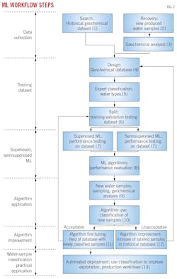
Fig. 2 shows workflow steps. Initial steps require compiling chemical-physical and elemental concentration measurements of produced water into a database derived from historical samples in a specific area or field. In cases where little existing historical information exists, the database obtains geochemical compositions from additional bottomhole or surface well samples from the field of study (Steps 1-4).

In Step 5, an SME classifies the samples into natural water (formation water) or production-related water (mud filtrate, completion brine, supply water, condensate water, or mixed water). Step 6 arbitrarily divides the dataset into a training and testing dataset (for example, 90% and 10% of the total samples, respectively). Supervised and semi-supervised ML training learns and tunes hyperparameters from the training dataset (Step 7).

Key parameters for recognition of different water types are identified through elemental ratios, such as Ca/K and SO4/Ba. The test-data subset compares algorithm classification performance (Step 8). The algorithm with highest performance classifies field-produced water samples based on their compositions (Steps 9 and 10). Quality control is overseen manually.

If the results are acceptable, the training set is expanded by including newly classified samples with geochemical fingerprints (Step 11). If results are unacceptable (discrepancy between SME and ML classification) the training set is extended by adding more control samples (Step 12). Once the ML model is trained, exploration and production models include water classifications produced by the model (Step 13).

ML testing

The ML workflow using XGBoost was applied to a geochemical dataset of 777 produced water samples from exploration and development wells. The set was arbitrarily divided into 700 samples for a training dataset with known water types for semi-supervised learning and 77 samples for a testing dataset to predict water types.

Elemental ratio most effectively separated water types. Detailed analysis of ratios from produced water samples and their assignment to water types revealed that Sr/K vs. Ca/SO4 comparisons distinguished formation water from mud filtrate, Ca/HCO3 vs. Ca/Cl comparisons discriminated formation water from condensate water, and HCO3/Br vs. Na/SO4 identified completion brine from formation water.

Comparing predicted water types with SME classifications determined ML model performance. The ML model correctly predicted water types for 70 samples out of 77, an 89.7% performance rate.

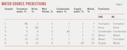
Table 2 shows model predictions for six selected samples against SME identification. The table shows percentages for brine, condensate water, formation water, mixed water, mud filtrate, and supply water with probabilities for each of these water types contributing to the overall composition of each sample. Green indicates samples with SME and ML agreement, and red indicates discrepancy.

Sample 1 had high NaCl content (47,483 mg/l. Na, 98,102 mg/l. Cl, 152,972 mg/l. total dissolved solids (TDS)) and was identified by both methods as formation water. For Sample 2, elevated K (5,220 mg/l.), Mg (20,228 mg/l.), and Br (31,505 mg/l.) concentrations were key indicators for the ML model to predict a brine origin. Low salinity (TDS = 621 mg/l.) indicated condensate water for Sample 3. Sample 4 was mixed based on depleted Na and Cl concentrations and the dominance of SO4 (4,395 mg/l.). The composition suggested that formation water had mixed with drilling fluids and diluted supply water, and both the ML algorithm and SME evaluation agreed.

Samples 5 and 6 show discrepancies between expert and ML-performed fluid classification. For Sample 5, the SME determined that the elevated HCO3 concentration (1,441 mg/l.) indicated a mixture of a minor fraction of supply water with NaCl-laden formation water. The ML model determined the sample was pure formation water with a probability of 70.4%.

Field application

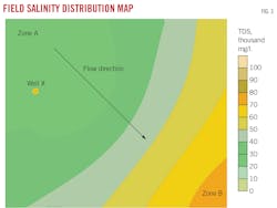
Fig. 3 shows a map of formation water salinity distributions within a gas field. The arrow indicates water migration direction. Salinity increases from Zone A in the vicinity of the outcrops towards discharge Zone B near the coast. TDS increases from 30,000 mg/l. in the northwest to about 80,000 mg/l. in the southeast, implying lateral fluid migration. Three water samples collected from Well X in the northwestern region showed markedly different characteristics from surrounding wells. Sample TDS concentrations varied between 68,540 mg/l. and 77,580 mg/l. (Table 3) and suggested restricted fluid migration and isolated hydrodynamic groups.

Field Salinity Distribution Map. Fig. 3.

To confirm this interpretation, the samples were analyzed using the ML workflow to identify water provenance and type. Table 3 shows probabilities of each water type’s contribution to the collected water sample composition. All samples suggest a high probability (above 85%) for brine from drilling or operational sources rather than from a natural isolated hydrodynamic group. The samples, therefore, are not representative of primary formation water and cannot be used as indicators for subsurface flow.

ML scaling tendency prediction

SLB developed an ML-based ROM to quantify physicochemical properties and scaling tendencies of oilfield waters as replacement for rigorous, first-principle thermodynamic models. Thermodynamic models provide the most accurate results and typically replace time-consuming laboratory experiments, but they typically require specialty training and are often difficult to integrate into digital workflows in the cloud or in edge computing near surface equipment or with downhole tools monitoring real-time well conditions. ROMs, by contrast, are fast, suitably accurate, and readily customizable to application.

ML model construction

Data to parameterize the ROM came from the US Geological Survey (USGS) produced waters geochemical database which originally contained 115,000 produced-water and other deep formation-water samples collected in the US in the past 120 years. Removal of inconsistent, poorly populated, and outlier samples resulted in about 85,000 verified records. Specific gravity (SG) was added to records from which it was missing based on Na, Ca, Cl ion concentrations and reported TDS, and concentrations were converted to mass percent to avoid concentration dependency on fluctuating sample density with temperature or pressure. Concentrations of K, Mg, HCO3, SO4, and Br ions were added when missing because they are always present even if missing in reports. Concentrations of minor ions or species (Sr, Ba, Fe, Zn, F, and H2S) were likewise added if missing from the record, but only to a randomly selected subset of the samples.

The USGS dataset was limited to only produced water in North America and analyzed under ambient conditions where precipitation could render them undersaturated over in-situ formation water. Principle component analysis (PCA) adjusted solute concentrations across a range of pressures and temperatures to produce 90,000 unique compositions as part of 1 million rows of pressure and temperature values to avoid concentration bias in such conditions.

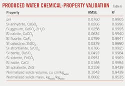
Saturation indices (SI) were calculated using Equation 1. SI require the ion activation product (IAP) and solubility product (Ksp) of the corresponding mineral. IAP depends on ion concentrations. Therefore, the dataset was amended to include 11 ion concentration products including NaCl and CaSO4 over large temperature and pressure ranges.

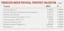
First-principle thermodynamic simulations were performed with commercial software using all PCA-adjusted database records for input, and the simulations produced 20 physicochemical properties including nonequilibrium (prescale) SI, precipitated minerals, evolved gases, and dissolved species. Total computational time was about 6 weeks for more than 1 million simulations.

The output was split between 80% of the simulations serving as a training set for the ML algorithm and 20% set aside for independent ROM validation. Root mean square error (RMSE) minimization optimized ROMs with 10-fold cross-validation.

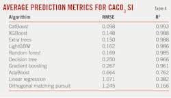
Model screening included 20 of the most-common machine-learning algorithms. RMSE and coefficient of determination (R2) for the models’ CaCO3 SI prediction are listed in Table 4. Decision tree algorithms CatBoost and XGBoost performed the best. These algorithms, however, require hyperparameter optimization (HPO) which can be computationally expensive. They also may quickly overfit and are sensitive to outliers. A workaround included stacking multiple weaker models, and this work used a hybrid approach with limited HPO followed by aggregating the resulting models. Model optimization depends on use case, and prediction accuracy may not be the primary objective if training and inference times, model size, and ease of deployment take precedence.

Average Prediction Metrics For CACO3 SI. Table 4.

For example, model runs with upper limits for hyperparameters and a maximum of 50 allowable trials produced results in about 2 hr training time per model with only 32 MB of model size. Table 5 shows high prediction accuracy (R2 > 0.9999) for eight produced water physical properties. SI and precipitated masses and volumes, however, are more difficult to model on first principles than these properties. The model accurately predicts pH, and since pH is a good predictor of SI, the workflow was improved to sequentially predict pH then refine SI and precipitate predictions based on predicted pH.

Produced Water Physical-Property Validation. Table 5.

Table 6 shows validation results for produced water chemical properties. Most properties have high R2 values (R2 > 0.99). For pH and most SIs, RMSE is a better metric for pH and SI, and was generally below 0.1, at which point prediction errors are similar in magnitude to experimental measurement error and exceed practical modeling requirements.

Produced Water Chemical-Property Validation. Table 6.

One exception was poor model accuracy for sphalerite due to its sparse appearance in the training set, low solubility product, and low concentrations masked by solutes with higher concentrations. Overall, the accuracy of the precipitate models exceeded typical flow-assurance requirements, but improved ROMs were developed for highly oversaturated systems from which several minerals precipitate simultaneously.

A web application was developed using an open-source library for Python that allows a user to enter water composition, select desired predicted properties, define temperature, pressure, and pH ranges, and quickly generate produced-water simulation results.