Neural network locates salt accumulations
Scott Morris
Tony Dupont
John D. Grace
Earth Science Associates
Long Beach, Calif.
A 3D geographic information system (3D GIS) directly loads and analyzes 3D seismic data for visualizing reservoir structure, pressure, depositional and paleo surfaces, wells, completions, logs, production, and other geologic and engineering data. Using the tool, a machine learning project analyzed large volumes of 3D seismic through 3D GIS over hundreds of 3D seismic surveys covering most of the Gulf of Mexico to identify salt. Most forecasted salts were in alignment with known salt locations from the training set.
Loading 3D seismic data
Loading and visualizing 3D seismic in 3D GIS advances the utility of GIS technology in exploration and production due to seismic’s fundamental role in reservoir and structural imaging. Continued advances in seismic-applicable spatial GIS tools further leverage that gain. This expansion of GIS technology fosters direct integration of vector well data (e.g., logs, pressure) and local-regional surfaces (e.g., paleo) with seismic surveys. It also expands the application of machine-learning techniques which access a variety of data sources.
The SEG-Y file format is the industry standard storage for seismic data. This format, however, stores data sequentially which is not beneficial for modern computing processes. Loading seismic data into 3D GIS, therefore, requires changing the data structure. The network common data form (NetCDF), originally devised for ocean and atmospheric data, stores multidimensional scientific data and works well for three-dimensional subsurface data. The universality of NetCDF provides a wider range of seismic data applications and efficiently loads in 3D GIS.
Conversion of seismic data to GIS-ready format has specific spatial requirements. First, the seismic must be depth migrated as a GIS places items in real-world locations and cannot use time as a spatial dimension. Additionally, the geodetic data must be transformed into a regular grid in geographic space. The 3D grid optimizes rendering of massive-sized 3D seismic data sets because the software is not required to track the absolute location of every single point. Even with these advantages, however, the data must be either split into multiple files or a sampling program must be executed. SEG-Y files can be up to tens of gigabytes (GB) spanning thousands of square miles. The present maximum limit of the mapping software is about 3 GB.
GOM visualization
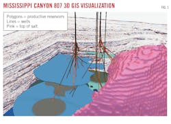
A study for the Gulf of Mexico migrated 3D seismic surveys in their native SEG-Y format and processed them for visualization with 3D GIS. Fig. 1 shows the seismic in a typical 3D GIS-field view for reservoirs in Mississippi Canyon 807 (Mars-Ursa) field looking to the west. Once the NetCDF was created, it was added to the 3D GIS scene as a voxel layer (multidimensional spatial and temporal information in a 3D volumetric visualization). In Fig. 1, the seismic has been sliced into a background, giving context to the field’s productive sands (3D polygons colored by estimated ultimate recovery), wells (showing resistivity log values), and the top-of-salt surfaces (pink).
The 3D seismic layer functions like any other in 3D GIS, except it has voxel layer-specific tools. The most important is Slice. It creates arbitrary cross-sections through the seismic data in any direction and orientation. The seismic cube can be peeled back to reveal various inline and crossline data throughout the survey. Typical GIS tools apply, like clicking on seismic data to show a pop-up window with associated data. There is also a hover functionality that displays the geographic and depth location of each point in the seismic.
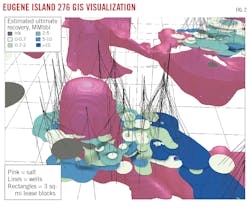
The black lines are boreholes, and the rectangles are 3-sq mile lease blocks. Estimated salt volume was extracted from the velocity model of the seismic survey. This analysis produced a regional salt volume (Fig. 2) which shows a salt dome responsible for organizing the accumulations of the Eugene Island 276 field (pink). Reservoirs between 6,500 and 11,000 ft are mapped as 3D polygons, colored to reflect estimated ultimate recovery. Wells are indicated by black lines. The dome rises above the field’s reservoirs to just below the seafloor.
The 3D GIS framework readily adds vector data (wells and reservoirs) and gridded surfaces of geologic variables (age, environment of deposition), or drilling information (pressure).
Machine learning
Rendering 3D SEG-Y into NetCDF and satisfying geodetic demands of a GIS prepares seismic for machine learning analysis. These requirements support analytic operations on the 3D seismic data which would be much more difficult if just relying directly on SEG-Y. The utility was tested by teaching it to identify salt.
Of more than 1,400 3D GOM seismic surveys available to the authors, a minority contained velocity surveys. A supervised machine-learning model was trained to classify each voxel in all surveys as salt or non-salt to produce 3D salt maps equivalent to Fig. 2 (which relied on velocity data). Taking the supervised learning approach to regional salt mapping is in contrast to previous work using unsupervised techniques applied to 2D seismic.1
Surveys with velocity data were filtered to records with velocity > 14,000 ft/sec. This became the training set for the location of salt in the survey. At each point classified as salt by velocity, a flag was added to the 3D seismic layer. For all locations outside estimated salt, the flag was set to non-salt. This set up a binary forecasting assignment (OGJ, Mar. 6, 2023, p. 22).
To address the former issue, amplitude values were normalized, as is standard practice in machine learning processes. The latter issue was solved by scaling surveys for uniform spacing between amplitude sample locations in all dimensions and matches between all surveys. This task was accomplished using existing scaling libraries as the seismic data stored as a NetCDF is already arranged as a three-dimensional matrix.
A convolutional neural network (CNN, specifically a U-Net) was then applied to the training surveys, equipping each sample with seismic amplitude data plus the velocity-based salt or no-salt flag. CNN divides the entire survey into 32 × 32 × 32 × 1 grid voxels, where the grid is spaced 64 ft apart and stores only one value (amplitude). Using the voxel cube, the CNN model accumulates patterns in amplitude of the surrounding voxels as they relate to whether a voxel is salt or non-salt.
The CNN transforms those patterns into predictions, which are assessed for accuracy based on a sample test-set held out of the original training. Examining errors in prediction, model parameters are updated relating cube amplitude distributions to salt and no-salt flags, and the data is reprocessed. An increasingly reliable salt-no-salt prediction machine builds from multiple passes through the training surveys. This analysis uses the Keras package in Python with an Adam optimizer and binary cross-entropy as a loss function (because it is a binary classification problem).
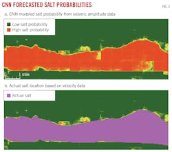
Fig. 3a and 3b compare early results between the distribution of salt based on velocity filtering (assumed to be “truth”) and the CNN salt or no-salt prediction for the same place. Fig. 3a shows forecasted probability for each voxel that is in salt. Salt is either present (red) or absent (green). There are some areas at the edges of the predicted salt that are equivocal predictions, but most forecasted values reflect a high degree of certainty in the support of binary classification.
Fig. 3b imposes the velocity-estimated boundary of the salt body as control. Again, there are disagreements, mainly at the edges. Actual salt nearly fully overlies the forecast, although there are a small number of false positives along the salt’s shallow boundary.
Reference
- Morris, S., Li, S., Dupont, T., and Grace, J.D., “Batch automated image processing of 2D seismic data for salt discrimination and basin-wide mapping,” Geophysics, Vol. 84, No. 6, Nov.-Dec. 2019, pp. O113-O121.
The authors
Scott Morris ([email protected]) is a mathematician at Earth Science Associates, Long Beach, Calif. He holds an MS (2012) in applied mathematics from California State University, Fullerton.
Tony Dupont ([email protected]) is chief operating officer of Earth Science Associates, Long Beach, Calif. He holds an MA (2009) in geography from California State University, Fullerton.
John D. Grace ([email protected]) is president of Earth Science Associates, Long Beach, Calif. He holds a PhD (1984) in economics from Louisiana State University. He is a member of the Society of Exploration Geophysicists, Society of Petroleum Engineers, and the International Association for Mathematical Geosciences.


