Smart gas lift unlocks value in shared well-pad comparison
Paul Munding
Flogistix
Oklahoma City, Okla.
Smart gas lift solves stable unloading problems by providing an integrated skid which includes its own programmable logic controller (PLC) for an integrated suction control valve, and an engine speed controller which communicates with its own injection meter. The machine can respond to dynamic source-gas conditions to maintain injection rate. Most importantly, it maintains injection above the minimum rate required to keep the well unloaded, avoiding heading flow.
Background
Gas lift operations have grown with increasing gas-liquid ratios (GLR) in unconventional wells. Gas lift effectively handles variable GLR and is largely impervious to solids such as sand and plug parts. It is, however, not as efficient as a mechanical pump for drawing a well down. Gas lift injection rates are typically set based on static design models, modified based on well performance, and statically set again until they are reviewed at some future time. This assumes that equipment responsible for injection will maintain constant rate.
Most small individual-well gas-lift compressors are less than 225 hp. Depending on manufacturing date, these units have a range of reliability heavily influenced by seasonal weather. Most small compressors built in the last 20 years have Murphy-type gauges, but without control automation. Whenever surface conditions change, operators and compression service company technicians actively maintain correct injection rates, but this drains key field personnel tasked with troubleshooting issues in order of priority on large oil production leases.
A smart gas-lift compressor that maintains proper injection rate and allows for remote control adds value in four areas:
- Increasing runtime from newly built self-monitoring and self-reporting machinery.
- Freeing up field personnel by allowing compressors to adjust themselves.
- Automatically adjusting rate to account for changes in line pressure.
- Increasing stable unloading by maintaining injection rate regardless of dynamic field conditions.
This article focuses on value derived from the last point.
Inability to maintain injection
A well that is down for less than 12 hrs may build a static liquid column equal to its bottom hole pressure (bhp) and subsequently log itself off. Therefore, it is imperative that production issues are addressed in a timely manner. However, this may be impossible when wells are far from the field office and nonautomated compression equipment requires on site diagnosis before taking corrective action. If insufficient gas is available to reduce fluid gradient, the well will slug and load up.
A suction control valve with a high-pressure setpoint is common practice for sourcing gas to a compressor, but the valve cannot regulate a standard, consistent suction pressure into the compressor below this setpoint. Given varying suction pressure, the corresponding varying compressed gas volume will lead to erratic injection, possibly less than stable unloading requires.
Stable unloading
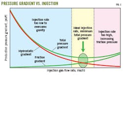
Gas lift is designed to lighten the fluid column to an ideal gradient from the lowest possible injection point where the well can unload fluid to surface with the highest possible drawdown (Fig. 1). Injecting gas greater than this amount can lead to increased friction and backpressure inside the production string. Conversely, injecting less than ideal gas volume results in a high gradient which cannot overcome the hydrostatic head. Overinjecting is preferable to underinjecting and is why a consistent daily supply of injection gas is critical. Discrepancies between models and well tests in lift-gas performance curves are often most pronounced at low injection rates, which is the region where accuracy is most needed.
For horizontals, multiphase flow instabilities become more pronounced once the well has transitioned from fracture dominated flow to matrix dominated flow. In most cases this occurs 3-9 months after initial production. Production curves tend to flatten during this period, known as tail production, and water cut increases as reservoir pressure decreases due to relative permeability effects.
Annular flow is the most efficient flow regime to produce these wells, in which the superficial gas velocity carries liquid to surface in the form of film and droplets (Fig. 2). If gas rate increases further, the regime transitions to mist flow, which comes with much higher frictional losses.

Slug-flow is the regime wells fall into on the path to loading up. Between slug and annular flow is churn flow which occurs at a small range inside standard 27/8-in. and 23/8-in. pipe.
Although annular flow is the most efficient, it is difficult to achieve in most oil wells. Churn flow, with oscillating motions of the liquid film efficiently carrying liquids to surface, is more practical for liquids removal.
With annular flow, about 5-10% of liquid is held up inside the pipe. Churn flow regimes have liquid holdup of 15-30%. Due to high GLR, horizontal oil wells most naturally unload with churn flow (in vertical) and pseudo slug flow (in horizontal) after being brought on production.
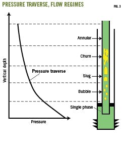
Various multiphase flow regimes may exist along an oil well from surface to bottom caused by release of solution gas and subsequent gas expansion as pressure drops (Fig. 3). With slug flow, liquid holdup may reach 40-50% inside pipe. Further slippage past slug flow creates bubble flow with 70-80% liquid holdup, during which bubbles ascend through a liquid column. Below that point, an oil well has a single-phase fluid column with gas in solution which puts backpressure on the formation.
Drawing a well down as far as possible requires proper amounts of injection gas to ensure annular or churn flow on bottom. Below this amount a well begins to load and exhibit heading flow as a single-phase hydrostatic liquid column rises and casing pressure builds. Rising pressure causes the check valve to close on injection-operated gas-lift valves, further building casing and tubing pressure and causing more liquid fallback until the well becomes static with no flow. Subsequently, a period of casing pressure buildup is required to reopen the valve.
When the valve reopens, injection gas blows through the valve and lightens the fluid column enough to produce a big column of fluid to the surface. The well then loads up and repeats the process. The difference between continuously producing a well in churn or slug flow and intermittently in heading flow is the ability to keep BHP constant. Under churn or slug flow conditions, BHP remains flat as drawdown is constant. Under heading flow, BHP builds, reducing inflow from the reservoir.
Oklahoma case study
Production installed a smart gas lift unit for one well on a two-well pad in southern Oklahoma. The other well had its own nonautomated reciprocating compressor. The compressors were pulling from the same gas supply.
Analysis of daily production trends monitored data for significant changes in flow rates. Cumulative production could not be used since the two wells came online at different times and had different reservoir deliverability. Casing pressures were compared to indicate whether the wells were maintaining constant BHP. Fig. 4 shows oil production from Jan. 1, 2019, to Mar. 31, 2019, and Fig. 5 shows casing and line pressure for both wells over this period.
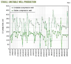
Line pressure is nearly identical for the two wells and averaged 85 psi, but there were nine events over a 3-month period during which line pressure rose above 100 psi for as long as several days. High line pressure impacts wells by increasing backpressure, decreasing drawdown and production. The smart gas-lift well (stable compression) quickly returned to trend versus the gas-lifted well on nonautomated compression (unstable compression). Another observable difference is large swings in daily oil rates in the unstable compression well, ranging from 4 to 450 bo/d.
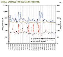
Low line pressure events, below trend, happened about six times over the 3 months, often followed by a high line pressure event. The low line events on Jan. 16, Feb. 6, Feb. 18, and Mar. 1 meaningfully impacted the well on nonautomated compression. The event on Jan. 16 caused the well to load up. The well exhibited 7 days of heading behavior as it was loading up, building pressure on the casing and then blowing to surface. This can be seen in both the oil production rate and casing pressure.
The second low line pressure event on Feb. 6 caused the well to load up, as observed by a drop followed by an immediate increase in casing pressure as fluid built up in the tubing. It took the well 4 days to reduce casing pressure to valve operating pressure. The low line pressure event on Feb. 18 also took 4 days for the well to reduce unloading casing pressure back to prior trend. The low line pressure event on Mar. 1 caused severe heading and slugging behavior that lasted 10 days before the well stabilized and unloaded from lower valves. The well using smart gas lift stayed unloaded after these events, with relatively stable casing pressure.
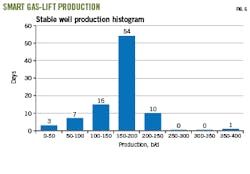
Figs. 6-7 show histograms of daily oil production and illustrate the erratic behavior in the nonautomated injection unit during upset compared with the smart unit. Production is split into 50-bbl bins. In Fig. 6, smart gas-lift daily production numbers are around 150-200 bo/d, while the next most populated bins are 100-150 and 200-250 bo/d. Fifty-four days of production are within the mean, representing 60% of production time. The next two closest bins represent 28% of the time. In total, about 88% of daily production falls within one bin of the mean.
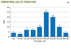
In Fig. 7, the histogram of the well gas lifted with nonautomated compression shows that the 250-300 bo/d mean bin has only five more daily occurrences than the 300-350 bo/d bin. The third highest bin is 150-200 bo/d at 12 occurrences, followed by a tie between 200-250 bo/d and 350-400 bo/d. Fifty-five days of production, representing 60% of time, falls within one bin of the mean as compared to 88% for smart gas lift.
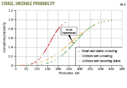
The 50-bo/d bin size is relatively large compared with daily average production, however, and a cumulative probability plot can provide finer analysis (Fig. 8).
The smart gas-lift production curve (orange) shows a tighter production distribution than the nonautomated compressor. For the latter, production is between 170 and 350 bo/d for 60% of the time, a broad range indicative of unstable unloading brought on by heading flow from insufficient gas injection rates. The smart gas-lifted production lies in a narrower range between 125 and 200 bo/d for 60% of the time.
The production potential of the nonautomated compressor well, had it been equipped with a smart system, was estimated by redistributing daily production percentages to match the shape of the histogram of the smart gas-lift compressor well. It represents the unstable well unloading like the stable smart gas lift system. The results of this histogram are plotted on Fig. 8 and show a tighter rate spread. With daily production following a more stable unloading pattern, the mean moves from 258 to 276 bo/d, a net 18 bo/d increase.
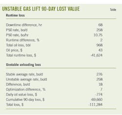
Besides the ability to unload the well in a more stable fashion, compressor run time was 2% better with the smart unit. Cumulative difference between both runtime and average daily oil production are summarized in Table 1, including losses that could have potentially been recovered had a smart gas-lift unit been used. In 3 months, $111,284 was potentially lost without a smart gas-lift compressor controlling rate.
Bibliography
Avest, D. and Oudeman, P., “A Dynamic Simulator to Analyze and Remedy Gas Lift Problems,” SPE 30639, SPE Annual Technical Conference and Exhibition. Dallas, Tex., Oct. 22-25, 1995.
Campos, M., Lima, M., Teixeira, A., Moreira, C., Stender, A., Von Meien, O., and Quaresma, B., “Advanced Control for Gas-Lift Well Optimization,” OTC-28108, SPE Offshore Technology Conference, Rio de Janeiro, Oct. 24-26, 2017.
Guner, M., Pereyra E., Sarica C., and Torres C., “An Experimental Study of Low Liquid Loading in Inclined Pipes from 90° to 45°,” SPE-173631, SPE Production and Operations Symposium, Oklahoma City, Okla., Mar. 1-5, 2015.
Jansen, B., Dalsmo, M., Nokleberg, L., Havre, K., Kristiansen, V., and Lemetayer, P., “Automatic Control of Unstable Gas Lifted Wells,” SPE-56832, SPE Annual Technical Conference and Exhibition. Houston, Tex., Oct. 3-6, 1999.
Kaasa, G., Alstad, V., Zhou, J., and Aamo, O., “Nonlinear Model-Based Control of Unstable Wells. Modeling, Identification and Control,” MIC Journal, Vol. 28, No. 3, July 2007, pp. 69-79.
The author
Paul Munding ([email protected]) is vice president of petroleum engineering at Flogistix LP. He holds a BS in petroleum engineering (2003) from the University of Oklahoma and has a professional engineering certification. He is a member of the Society of Petroleum Engineers.