Regressions allow development of compressor cost estimation models
View Article as Single page
Cost estimation
The data set collected in this study has information on compressor station capacity and location as well as individual cost components. Researchers studied the multiple nonlinear regression methods used to assess pipeline cost data (OGJ, July 4, 2011, p. 22).6 This study, after trying different regression models, used the general form of multiple nonlinear regression model shown in Equation 1.
The Central region is the cost estimation base case. S denotes compressor station capacity, αi is the coefficient of variables (i = 0,…6). Positive αi of regional variables shows the region has a higher cost than the Central region cost, while negative αi (i = 0, …5) of regional variables shows the region has a lower cost than the Central regional cost.
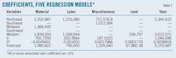
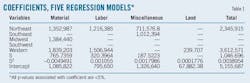
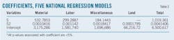
Researchers used this approach and available data to develop five cost estimation models. Table 1 shows coefficients of the regression models. National regression models developed for five individual cost components assigned the coefficient of regional variables as 0. Table 2 shows the coefficient of the regression models.
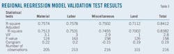
The corrgram test examines residual autocorrelation.7 Table 3 shows the maximum value of autocorrelation from Lag 1 to Lag 40. Autocorrelation lies between –0.17 and 0.22. Results show errors associated with observations as statistically independent from one another.
Researchers used an F test and its associated p-value to test the overall model for predictive capability. The name of the ratio of the square mean of the square for regression and the mean square for error is F-statistics.9 Normally a large F-value suggests the model explains a large proportion of variance. The p-value associated with the F-statistic is significant when the p-value is less than 5%.
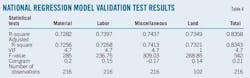
F-statistics of all five models are very large and associated p-values are less than 1%, leading to the conclusion that at least one of the model’s parameters has predictive capability. All p-values of coefficients measuring well below 5% allows the conclusion that parameters in all 10 models are significant.
R-square and adjusted R-square help determine the model’s goodness of fit. R-square shows the independent variables explaining the proportion of variance in the dependent variables. One disadvantage of R-square is that its value can be artificially inflated by putting in additional independent variables.10 Adjusted R-square, therefore, usually accompanies R-square when determining fit.
The values of R-square for all models are greater than 0.71, and the adjusted R-square values are almost the same as the R-square values in all models, showing that a large proportion of variability in the model can be explained by the independent variables and that these regression models are good models.
Various diagnostics and tests, therefore, validate these 10 regression models. The following section uses these regression models to analyze cost differences in regions and compressor station capacities.
Displaying 2/5
View Article as Single page