Vibration modeling improves pipeline performance, costs
Ben Rahmoune Mohamed
Ahmed Hafaifa
University of Djelfa
Algeria
Guemana Mouloud
University of Medea
Algeria
Modeling neural networks to vibration patterns of operating gas turbines and then applying these models to the same turbines' future performance and maintenance can reduce costs and improve operations.
Industrial monitoring increases the reliability of plants and processes, including gas turbines. Turbine vibrations can degrade the unit's working condition and be symptoms of future failure. Their continuous operating state places a premium on quick and early detection of problems. Doubling or tripling the number of sensors, however, substantially increases costs and can create both hardware and software congestion.
There are two general approaches to monitoring: quantitative, mainly using analytical models (parity space, observers, parameter estimation, etc.); and qualitative, using methods without analytical models (based primarily on techniques of artificial intelligence).1 This article discusses the use of a neural network to examine vibrations of a gas turbine. The network can learn vibrations in an operating gas turbine and use them to help design future networks used to plan preventive maintenance.
Examined system
The GE MS3002 gas turbine at the Hassi R'mel gas plant in southern Algeria (Fig. 1) moves residual dry gas into the Algerian pipeline network for eventual shipment to Europe via sub-Mediterranean pipeline. The turbine system has machine-driven dual overhead mechanics and simple-cycle construction consisting of an axial compressor, 15 floors, 6 combustion chambers arranged at 90° angles, an axial intake, a single high-pressure turbine stage (first stage) driving the compressor and its auxiliary equipment, and a low-pressure turbine (second stage) that drives the load. The turbine assembly consists of three main elements: axial compressor, combustor, and turbine.
The first step in diagnosing the turbine is to choose a neural model, the second step is to generate residuals, and the third to decide a course of action to address localized defects. The choice of the neural model in learning to identify the turbine's dynamic behavior depends strictly on the complexity of the state, comparing healthy functioning with malfunctioning, used to generate a neural model. This study modeled the turbine's behavior, using a "feed forward" network type and the multilayer perception (MLP) model.
Industrial processes are often complex systems with strong nonlinearities in their operation, which cause problems in controlling these systems and require the operator to formulate a workable model. Linear techniques around an operating point or order reduction can mathematically model performance degradation of a real system.
Retro-spread of the gradient of the error as a learning algorithm in the neural structure most commonly used for modeling algorithm retro-propagation of the error gradient can solve the problem of calculating the errors of the outputs of the hidden layer neurons. Each of the training sets, for example, contains back propagation algorithms consisting of two phases:
• Propagation, during which the corresponding entries are used to compute the outputs of all neurons.
• Reverse, in which the gradients are calculated or are local errors for all neurons.
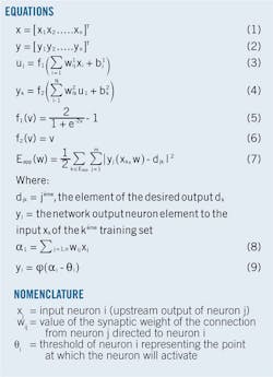
The network parameters for input vector and output vector can be written as shown in Equations 1 and 2, respectively, in the accompanying box. Equations 3 and 4 show the general law for calculating the outputs of neurons of the hidden layer and the output layer, respectively. Equations 5 and 6 provide the linear and sigmoid activation functions.
The learning algorithm by the back-propagation gradient error, or any short back-propagation algorithm, provides the basis for adjusting the physical process's weight vector to minimize the quadratic cost function defined by Equation 7.
Two phases model behavior of the artificial neuron:2
• A summation operator, which develops the potential, a. This operator performs the weighted sum of the inputs by subtracting the sum of both the activation thresholds, θi.
• A nonlinear operator, which calculates the value of the activation. This operator is called the transfer function.
Weight indicates a positive effect of an excitatory transmitter neuron (j) to the receiver neuron (i). A negative weight has an inhibitory effect. The function generates the combination of the inner product vector and input vector of the synaptic weights, calculating the weighted sum of the entries, according to Equation 8.
From this value a transfer function (or activation-thresholding function), φ, calculates the value of the neuron state. Equation 9 transmits this value to the downstream neurons. The most frequently used values are those for which φ is a nonlinear function, typically the hyperbolic tangent of a linear input.
Modeling results
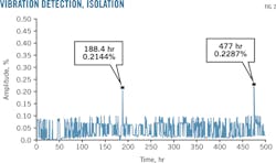
Table 1 represents the architecture modeling of the examined gas turbine system after modeling of its data system. The training set of the neural network looks for the best settings of those that scored closer than the mathematical model based on real data of the examined gas turbine. Detecting and locating faults set vibration ≥ 0.1% amplitude as the maximum tolerance (Fig. 2).
Vibrations in the gas turbine can cause damage, leading to high maintenance costs, lack of reliability, and potentially replacement of the entire turbine. Predicting vibration, however, can mitigate against these consequences. Building a neural network matching the curves of the actual devices drives this prediction. Table 2 shows model values for given time increments.
The prediction model's output () schedules the maintenance plan (Table 3), reducing the costs of future intervention.
References
1. Hafaifa, A., Mouloud, G., and Attia, D., "Fault detection and isolation in industrial systems based on spectral analysis diagnosis," Intelligent Control and Automation Journal, Vol. 4, No. 1, February 2013, pp. 36-41.
2. Yang, S. H., Chen, B. H., and Wang, X. Z., "Neural network based fault diagnosis using unmeasurable inputs," Engineering Applications of Artificial Intelligence, Vol. 13, No. 3, March 2000, pp. 345-356.
The authors


