Technique connects known, unknown EURs, manages expectations
Doug Tierney
Encana Services Co. Ltd.
Denver
Reserves reports often rely on volumetric probabilistic EUR assessments while remaining vague or silent on how these estimates relate to what is actually known or proven. In some respects, they avoid reporting on fully risked volumes. The consuming audience should be cautious about assuming these reports represent expectations. Doing so may lead to serious overstatement or confusion regarding expectations. Rather they are probabilistic output from geoscience exercises fraught with assumptions. Often, there is a clear need to reconcile various sources of information so that stakeholders can coalesce around a robust, shared view of resource potential.
The examples contained here address a few of these issues, as well as demonstrate a useful technique to render reasonable expectations across a broader range of uncertain outcomes associated with newer and emerging fields or plays.
A logical graphical technique connects known and unknown EUR figures properly to manage expectations, along with a few practical examples. Governed by the central limit theorem, the idea is that expected ultimate recovery size range for a prospect should be lognormal.
Managing expectations
Upon establishment of commerciality, however, there are volumes of remaining recovery for which the evaluator should be absolutely certain (the known). When these certain volumes are added to a lognormal resource size distribution (RSD) of what remains-to-be discovered or proven (the unknown), the resulting curve will exhibit downward concavity; that is, it is no longer lognormal.
The technique involves six primary steps:
• Step 1. Determine what ultimate recovery is known with absolute or near-absolute certainty. If a current and credible proved reserve figure is available, the known value should be somewhat lower, as proved reserves only need to pass a "reasonable certainty" test, typically around the 90th percentile (P90).
• Step 2. Determine the maximum expected EUR. In the parlance of exceedence probability, this is the P1. In practice, this number should be uncomfortably large because there is 99% certainty the ultimate recovery will be less than this figure. P1 is rarely mapped and commonly extrapolated from rigorous volumetric assessments with which geoscientists are more comfortable.
• Step 3. Subtract the known figure from the P1 EUR determined in Step 2. This is the P1 of what is yet-to-be discovered or proven over time.
• Step 4. Determine a small but practical yet-to-be discovered volume beyond the known figure. As we will be working on a log scale, it is impractical to assume very small numbers. The choice should be within the fidelity of the known figure but adequately small to represent the unknown P99.
• Step 5. On lognormal-probability paper, plot the P99-P1 line from the points to describe the RSD for what is unknown (yet-to-be discovered or proven).
• Step 6. Add the known figure to the unknown RSD to calculate the EUR expectation curve.
Note that choosing the points for Steps 1, 2, and 4 is subjective, and in practice this is where art meets science.
When you finish these steps, the efficacy of the method should be tested. For instance, calculated remaining recoverable resource-to-production ratios (R /P ratios) should be commensurate with appropriate probabilities. If a credible and current proved reserve figure is available, it should intersect the curve at a percentile that is "reasonably certain," somewhere around P90. If the resulting curve is unreasonable, the input assumptions should be revised and the process repeated.
Expectations of EUR are dynamic over time. As more information is gathered, the EUR-RSD curve will change. Typically, this change occurs from testing and condemning certain ideas that reduce the upper end of the curve. On the lower end, ever increasing cumulative production and rigorous updates to the proved reserves assessment provide increases in EUR.
Next are a few examples to demonstrate the application of the technique.
Application
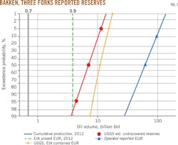
In the Bakken play, there are multiple sources of reserves and resources (Fig. 1). US Energy Information Administration (EIA) and US Geological Survey (USGS) figures were published with an effective date of yearend (YE) 2012, which is noted for reference.1 2
More recently, an operator published data that is much larger than the government published figures.3 The numbers differ, which is common and understandable for different evaluation vintages, as do the context, opinions, and biases of the evaluators. Confirming which estimates are correct could take another decade, but plotting the information allows us to make a few quick observations:
• The USGS appears 98% sure the proved reserves for the play will double.
• Neither curve represents much variance, with a P10/ P90 ratio of 2-3. This implies that both evaluators were very confident of their input assumptions, but the curves do not intersect nor overlap.
• Linearly extrapolating the operator's data would suggest there is a 97% chance this play will ultimately produce at least as much as the YE 2012 (EIA and USGS) proved US reserves of 33 billion bbl of oil.1
• The operator's data also suggest with high probability that this play could be double or even triple the YE 2012 proved reserves for the entire US.
These points are confusing and seem to include brave assertions and contradictions. The two unproven curves indicate that proven reserves are unreasonably certain; that is, it is absolutely impossible that ultimate recovery ends up that low. Nor do the lines overlap, which implies that neither evaluator's assumptions are considered remotely possible by the other (or perhaps this is why the operator was enigmatic by not publishing a P90 figure).
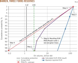
The described technique can provide some clarity and continuity to expectations across a full range of possible outcomes (Fig. 2). The following steps are color coded in Fig. 2:
• Step 1. For the known value (green line), consider that by mid-2014 the play had already produced about 1.2 billion bbl of oil, and the production rate of 1.1 million bo/d was still growing monthly by 20,000 bo/d.4 5 By the end of 2014, the play should easily top 1.3 billion bbl of oil and will not yet be in decline, nor will the drilling inventory be exhausted. To account for this, we can double that figure for a known volume of 2.6 billion bbl of oil.
• Step 2. Because the 137 billion bbl of oil number extrapolated from the operator's published data seems large,we can use that as P1.
• Step 3. The difference of 134.4 billion bbl of oil serves as the P1 of the yet-to-be discovered or unknown RSD.
• Step 4. The number 0.2 billion bbl of oil seems adequately small as the unknown P99 for this exercise. This number represents 6 months' production at the mid-2014rate.
• Step 5. Refer to Fig. 2 for the plot of the resulting unknown RSD.
• Step 6. Refer to Fig. 2 (red line) for the result. Using this technique, we now observe P90-P50-P10 expectations of 3.5, 7.5, and 34 billion bbl of oil, respectively, from the purple curve.
It is important to then check these numbers for reasonability. The EIA proved figure of 3.9 billion bbl of oil intersects the curve at the 87th percentile,which is very close to P90 and passes the "reasonably certain" criterion, perhaps even conservatively. If this outcome is a concern, the process could be repeated with a somewhat higher known value.
The P50 expectation is 8 billion bbl of oil (double theproved figure), which again seems reasonable for this play and is more conservative than the P50 values reported by the other entities. When computing R /P ratios, the described technique yields 6, 16, and 82 years at the P90-P50-P10 percentiles. Again, the 6 years at the P90 level appears low for this growing play, and if more rigor or accuracy is desired the process could be repeated.
The EIA published YE 2013 figures in December 2014, and the Bakken proved reserve EUR has grown by 2.0 billion bbl of oil to sit now at 5.9 billion bbl of oil. This intersects the "old" expectation curve at a 65% chance of meeting or exceeding.
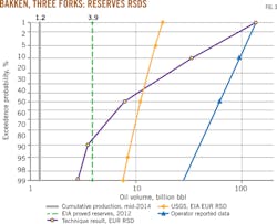
To wrap up this example, Fig. 3 plots the three EUR RSDs for comparison. The comparable R /P ratios from the previously published points are 152 and 227 years (P50 and P10) for the operator and 18, 24, and 39years (P95-P50-P5) for the USGS and EIA EUR-RSD. The EUR from the operator's publication was based on arigorous geoscience exercise and may ultimately be realized. For now, most stakeholders would be more comfortable with the expectations calculated from the technique presented here.
New discoveries
An operator recently reported successful shale-oil tests from vertical holes at a new discovery in Colombia and subsequently reported unrisked expectations from the play (limited to its gross acreage position).678 The company explicitly noted that the published figures were not adjusted for geologic risks. The published report covered multiple zones in three different blocks, which provides many permutations for successes and failures.
In the absence of information for a full-blown, risk-tree, or Monte Carlo assessment of the discovery, we can quickly apply the described technique to assess risked possible outcomes.
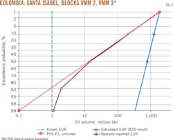
• Step 1. As a new discovery, the known value is essentially zero. We will assume 1 million bbl of oil for convenience on the log scale. Admittedly, this is a bit arbitrary, but the operator has secured farm-in commitments for 19 wells from three major oil companies; so it is not a stretch even if the play were determined noncommercial.
• Step 2.Extrapolating the operator's reported RSD to the P1 percentile yields 1,830 million bbl of oil.
• Step 3. Subtracting the known value yields a P1 for the unknown line of 1,829 million bbl of oil (essentially the same figure).
• Step 4. 0.1 million bbl of oil seems reasonable in this instance for the unknown P99 yet-to-discover resources in excess of the known figure.
• Step 5. Refer to Fig. 4 for the plot.
• Step 6. Refer to Fig. 4 for the result. Using the technique, we now observe P90-P50-P10 expectations of 2, 15, and 210 million bbl of oil, respectively. EUR is highly uncertain, and the results curve spans three log scales.
In this case, for which there are essentially no proved reserves, the technique gives us a general scale of magnitude. Therefore, if the play fails, there should still be a few million barrels recovered as different ideas are tested in different areas with the commitment wells. We should expect at least tens of millions of barrels to be produced, and about a 1-in-5 chance it exceeds 100 million bbl of oil. If it works well, it could exceed 1 billion bbl, but it is premature to assume this level of recovery.
Prediction, evaluation
Lognormal probability plots are useful tools for assessing the range of future outcomes. After commerciality is established, however, the EUR-RSD is no longer lognormal. Endpoints are important and should be tested for reasonability.
The described technique can bring clarity and continuity to expectations while bridging the gap between what is known and what is unknown yet possible. The technique is not a substitute for rigorous geoscience; indeed, applying rigorous geoscience to define probabilistic volumetric outcomes is a very useful input to help define the expectation curve.
EUR and similar reports are inherently subject to the bias of the evaluators. Expectations are dynamic and can dramatically change as new data are acquired. Caution is advised when adding resources or reserves reported from different sources.
For various stakeholders such as investors, policy makers, development planners, and regulators, application of this technique can help evaluate economic and social impact expectations and strategies to deal with possible outcomes. This technique may even help assuage conf licting views to provide consensus among opposing stakeholders.
References
1. US Energy Information Administration, "U.S. Crude Oil and Natural Gas Proved Reserves, 2012," April 2014, pp. 2-11.
2. Gaswirth, S.B., et al, "Assessment of Undiscovered Oil Resources in the Bakken and Three Forks Formations, Williston Basin Province, Montana, North Dakota, and South Dakota, 2013; USGS Fact Sheet 2013-3013," April 2013.
3. Continental Resources Inc., "Mapping our Future," Investor and Analyst Day Presentation, September 2014, p. 20.
4. Department of Mineral Resources, North Dakota Industrial Commission, Historical production statistics, https://www. dmr.nd.gov/oilgas/stats/historicalbakkenoilstats.pdf.
5. Montana Board of Oil & Gas Conservation, Historical production data, http://bogc.dnrc.mt.gov/WebApps/DataMiner/.
6. Canacol Energy Ltd., "Canacol Energy Ltd. Tests 590 BOPD From Fractured La Luna Formation Discovery at Mono Arana, Colombia," Press release, Mar. 6, 2014.
7. Canacol Energy Ltd. "Canacol Energy Ltd. Receives Prospective Resources Report for3 Shale Oil Blocks in the Middle Magdalena Basin, Colombia," Press release, Oct. 14, 2014.
8. Canacol Energy Ltd., "Growth from a Diverse Portfolio," Annual report, October 2014, pp. 11-12.


