Corrected maps narrow compressor performance prediction range
Haijun Chang
Changchun Wu
Xiaorui Zhang
China University of Petroleum
Beijing
Tests on two in–service compressors show corrected performance maps can predict a compressor's performance within 5% relative error under most situations. The correction is accomplished by moving the original performance map to best fit the compressor's performance data as deduced from operation records.
Centrifugal compressor performance will deviate from its performance map for a variety of reasons, including age, corrosion, and contamination. This article proposes a field–data driven method to correct this, moving a compressor's original performance map to best fit its records–deduced performance data and solving two least–square problems in this fitting procedure.
Testing on two in–service compressors on the Central Asia–China gas pipeline showed that the corrected performance map can estimate compressor performance within 5% relative error in most cases.
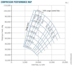
Performance maps typically supply centrifugal compressor performance data. Fig. 1's horizontal axis shows the volumetric flow rate under the compressor's suction condition and the vertical axis denotes the polytropic head. Fig. 1 also shows the equal–efficiency curve and equal–speed curve.
A compressor's performance map shows its performance under new and clean conditions. After operating for a period of time, however, a compressor's performance will deteriorate. Even after a full overhaul, a compressor will rarely retain its original state.
Retesting and redrawing a field compressor's performance map is uneconomic, time–consuming, and tedious. This article will instead use a historical–data driven correction method to acquire a compressor's changed performance map quickly and easily, testing it on two different compressor types.
Characteristic calculation
A compressor's operating records—including temperature and pressure data at intake and outlet, mass flow rate, speed, natural gas composition—are essential in obtaining a compressor's polytropic head and polytropic efficiency. Reasons such as measurement equipment failure can cause errors among these data. A simple filter tackles these errors.
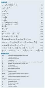
Using operational records data, Equation 1 yields a compressor's polytropic head. Equation 2 calculates the polytropic exponent item, mV. An equation of state such as the Benedict–Webb–Rubin–Starling (BWRS) equation, adopted throughout this article, or the AGA–8 function, can deduce the compressibility factor, Z.
Equation 3 yields a compressor's polytropic efficiency.1 The numerator is its polytropic head and the divisor denotes the natural gas's enthalpy difference at the compressor's suction and discharge. The American Petroleum Institute (API) procedure calculates natural gas enthalpy under specified temperature and pressure.2
Error filter
The head and efficiency data extracted from a compressor's operational records provide its actual performance, with four kinds of errors defined for data filtering and compressor–characteristic curve correction. The difference between the performance obtained by Equations 1 and 2 and the one forecast by its original performance map defines the absolute error (Equations 4–5). Equations 6 and 7 calculate relative errors.
A variety of errors may exist among a compressor's operational records. Removing erroneous data from the records manually is extremely time–consuming and ineffective. Filtering based on mistake patterns could also be inefficient because the number of these patterns could be very large. A simple operational records filter, however, can sort these data given some knowledge of their statistical properties. Given the large amounts of data for the same parameter, those lying far away from the majority are more likely to be erroneous, providing the basic idea for designing the operational records filter.
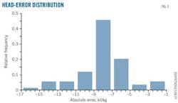
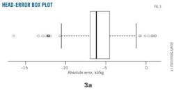
The error calculated by Equations 4–7 typically spreads widely, like the situation shown in Fig. 2: the distribution of a compressor's absolute–head error. The absolute value ranges from <2 to nearly 16 kilojoules (kJ)/kg, while the head value is 34–57 kJ/kg. Fig. 3 plots these error data by box plot. The three vertical lines in the middle that make a rectangle are the lower quartile, with the medium and the upper quartiles lying to the left and right, respectively.
The lower quartile splits off the lowest 25% from the highest 75% of the data; the medium cuts the entire data set in half, and the upper quartile splits off the tallest 25%. The distance between the upper and the lower quartile is defined as interquartile range (IQR).
Equations 8–9 define lower quartile (LB) and upper quartile (UB). The vertical line on the far left of Fig. 3 denotes the minimum point bigger than LB in the data set, while the straight vertical line on the far right represents the maximum point smaller than UB in the data set. The points beyond these two lines are outliers.
An outlying point is not necessarily erroneous but does have a much higher probability of being wrong and is therefore treated as bad and filtered out. Parameters adopted to filter operating records include absolute error of head and efficiency and corresponding relative errors.
Fan laws
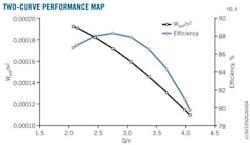
Fan laws describe a compressor's two operational points as shown in Equations 10–12. With this, a compressor's performance map can be reduced to two curves (Fig. 4). The horizontal axis denotes a compressor's volumetric flow rate under suction condition divided by its speed. The left vertical axis shows the corresponding polytropic head divided by the square of its speed and the one on the right its efficiency.
Fig. 4 shows that a compressor's performance map can be regressed in the form of Equations 13–14, in which the coefficients ai and bi (i = 0, 1, 2, 3) are compressor specified and obtained by regressing a compressor's performance map.
Map correction
The basic idea in correcting a compressor's performance map is to move it along the two axes shown in Fig. 4 to match the operation–records deduced data. Equation 15 shows the correction effects when the distances to move along the horizontal and vertical axes in positive direction for a compressor's head performance are Xhead and Yhead, respectively.
Calculating Xhead and Yhead requires solving a least–square problem (Equation 16), in which N denotes the quantity of filtered operation records and the subscript i is the counter. The item stands for the polytropic head calculated via the ith operation record. Provided a centrifugal compressor's speed is fixed, its polytropic head will decrease as its suction volumetric flow rate increases. This relationship suggests a constraint for Xhead because physics laws would be violated if Xhead is too high. Yhead calculations occurred without a constraint.
A compressor's efficiency performance map can also be corrected. Equation 17 shows the revised equation. Obtaining the corresponding movement values Xeff and Yeff, requires solving Equation 18 with no constraints on Xeff and Yeff.
Performance map correction can be summarized as follows:
- Regress a compressor's performance map with Equations 13–14. Digitalization is sometimes needed.
- Acquire the compressor's operation records, including its suction temperature and pressure, discharge temperature and pressure, speed, and natural gas mass flow rate and composition.
- Calculate the compressor's polytropic head and efficiency with its operation records according to Equations 1–3.
- Deduce the compressor's ideal polytropic head and efficiency by its performance map and operation record, including its suction temperature and pressure, speed, and natural gas mass flow rate and composition.
- Filter the operation records according to the performance errors defined in Equations 4–7.
- Split the filtered operation records into two parts. Use one of them in the correction procedure and retain the other for validation, naming the data sets accordingly. Their proportion in this article is 6:4 and their content is chosen randomly from the whole data set.
- Determine performance map correction items Xhead, Yhead, Xeff and Yeff by solving Equations 16 and 18 with the correction data set. If results show that the corrected polytropic head performance and its volumetric flow rate increase at the same time under any fixed speed, extra limits should be introduced to Xhead to eliminate this.
- Validate correction by analyzing differences between the actual performance and that predicted by the corrected performance map.
Fan–law reality
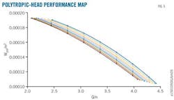
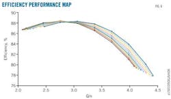
A single–stage compressor in a low–density environment observes fan laws perfectly. Multi–stage compressors, however, or large–diameter single–stage compressors allow application of fan laws only for small changes in speed.3 Figs. 5–6 show the performance map as a family of curves instead of a single one, with different colors representing distinct speeds.
A regression test shows that Equation 13 introduces considerable error, which could also be deduced from Fig. 6 in which the lines clearly separate. Equation 19, with more coefficients introduced to measure the influences of speed change on the coefficients a0, a1, and a2, can instead regress a compressor's head performance. The test also shows a moderate error in Equation 14. In the plot, however, the lines stay close enough to each other not to require any changes to the equation.
Changing the regression equation does not influence the correction method. Any other form of equation could be introduced to substitute for the current ones.
Tests
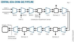
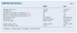
Testing of this method took place on in–service Central Asia–China gas pipeline compressors. Fig. 7 shows the 30–billion standard cu m /year (bcmy) pipeline's topology. The system uses two parallel 42–in. OD pipelines, with three input points, four delivery points, and eight compressor stations. Tests occurred on compressors at stations WKC2 and CS6. Table 1 provides some detail of the two stations and their compressors.
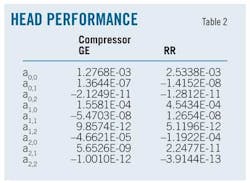
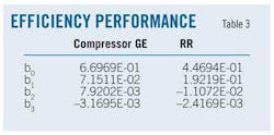
Regressing the compressors' performance maps yielded the results shown in Table 2 and Table 3, collecting, processing, and filtering operation records from October 2012 to May 2013.
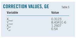
Test A focused on the GE compressor. Operation records after filtering numbered 128. Table 4 shows the sums of absolute–error squares before and after correction. Table 5 shows the correlation value.
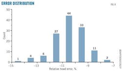
The sum of absolute–error squares decreases dramatically for the head performance. Fig. 8 plots the relative error distribution before correction. The horizontal axis denotes the relative error, and each column corresponds to a range of 1%. The number on the top of the columns shows the number of records in that range. Relative error ran to –15% and centered in the range of –13% to –8%.
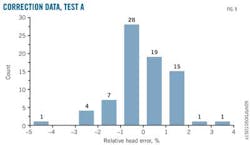
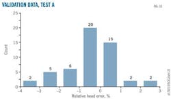
Figs. 9 and 10 show the corresponding relative error distributions for the correction data set and validation data set, respectively. Relative error is much smaller and overfit phenomena aren't seen.
The sum of absolute–error performance efficiency for squares doesn't decrease as much as it had on head performance. The relative error distribution before correction ranges from –1% to 5%, strongly suggesting the original efficiency performance curve is still accurate.
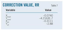
Test B took place on the Rolls–Royce compressor. Operational records after filtering numbered 88. Table 6 shows the sum of absolute–error squares before and after correction. Table 7 shows the correction value.
The sum of absolute–error squares for head performance decreases but not by as much as it had for efficiency, for the same reasons seen in Test A. The original head performance curve is still accurate enough. The relative error distribution of efficiency ranged as high as 18%, with the majority spread from –2% to as much as 14%.
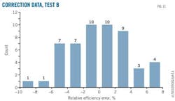
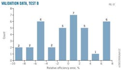
Figs. 11 and 12 show relative error distribution of the correction data set and the validation data set, respectively, after correction. Although the effect is not as close as it was in Test A, most of the error distribution is still –5% to 5% and accurate enough for engineering use.
References
1. "Performance Test Code on Compressors and Exhausters," PTC 10–1997, American Society of Mechanical Engineers, New York, 1997.
2. Danner, R.P., and Daubert, T.E., "Technical Data Book –Petroleum Refining," American Petroleum Institute, Division of Refining, 1983.
3. Odom, F.M., and Muster, G.L., "Tutorial on Modeling of Gas Turbine Driven Centrifugal Compressors," PSIG Annual Meeting, Galveston, Tex., May 12–15, 2009.
The authors
More Oil & Gas Journal Current Issue Articles
More Oil & Gas Journal Archives Issue Articles
View Oil and Gas Articles on PennEnergy.com
