Risk-based pipeline routing improves success probability
A project performing pipeline-risk mapping of the Persian Gulf region using a geographic information system has validated an early emphasis on risk management in making pipeline routing decisions.
Regional and global demand on the Persian Gulf's hydrocarbon reserves has increased dramatically in the last decade, and new pipelines will be needed to carry these reserves to market. Construction costs for Persian Gulf pipelines can easily exceed $1 billion and problems associated with the region's high-risk environments can lengthen project schedules and increase life-cycle costs.
This article validates the concept that a risk-management process, when applied through a geographic information system, can yield reasonable and economically viable pipeline alignments.
Additional goals of the project underlying this article included creating pipeline risk maps for the Persian Gulf region by identifying appropriate risk factors and weighting these by use of three common methods and testing the results against existing pipelines.
Risk-based approach
Projects incorporating a risk-management plan often carry cost and time savings. Although these plans are simply part of an overall project plan, rather than providing the project's primary framework, examples exist of successful projects in which risk mitigation itself was the goal.
Overfield and Collins describe a risk-based method for designing floating production, storage, and offloading vessels so that as reliability improves risk is reduced.1 Oliver and John use uncertainty modeling to develop a risk-based approach to pipeline corrosion monitoring and integrity management (OGJ, Nov. 5, 2007, p. 92). Dey et. al. developed a risk-based model for the maintenance of cross-country pipelines.2
Approaching the problem of pipeline route selection with a risk-based method has several advantages. Most project team members, regardless of background or experience, can develop a risk-management plan and adequately evaluate their project's risks, allowing route planning to proceed even if staffing shortages or other issues result in the absence of subject-matter experts during a project's early stages.
Many approaches described in the literature emphasize construction cost and related factors as primary route selection criteria. The risk-based approach described in this article allows for consideration of operational costs as well, thereby allowing a greater focus on life-cycle costs. Intangible factors can also be considered, making it possible to optimize the pipeline route to avoid environmentally sensitive areas or minimize exposure to areas of seismic activity.
Tools, data
Spatial analysis for this project was conducted with Environmental Systems Research Institute's (ESRI) ArcGIS 9.2 software, with heavy reliance on the spatial analyst extension. Complying with internal data security measures requires all spatial and tabular data used be taken from public online sources, including the Global Seismic Hazard Program, the National Center of Ecological Analysis and Synthesis, Reefbase, the United Nations Environmental Program GEO Data Portal, and the US Geological Survey. Data-quality issues involving resolution, accuracy, usefulness, and vintage may have affected results.
Risk factors
Literature review identified 36 pipeline risk factors (OGJ, May 29, 2000, p. 68, and June 22, 1998, p. 63),3-5 mapped throughout the study area shown in Fig. 1. Of these, 19 were terrestrial, 11 marine, and 6 covered both environments. There were no examples of GIS-based marine pipeline projects from which to derive route selection risk factors, making it likely some important marine risk factors were omitted from the potential-risk list.
Table 1 shows these risk factors divided into four categories for conceptual and analytical purposes: construction, operation, socioeconomic, and environmental. A formal risk analysis identified high-priority risk factors.
During a formal risk analysis, project team members evaluate each risk factor and assign probability of occurrence (PO) and potential impact (PI) scores of 1 (low), 2 (medium), or 3 (high). This project added the additional step of calculating a risk score (RS) for each risk using the formula (PO/2) + PI = RS, yielding a range of scores from 1.5 to 4.5 in 0.5 increments. Higher RS values show higher perceived risk.
This formula gave greater weight to the PI score, which allowed all risk factors with a PI of 3, regardless of their PO score, to make the minimum 3.0 RS cutoff established by the author for high priority risks. The formal risk analysis identified 21 high-priority risks, but data availability issues reduced this list to 20.
Weighting methodology
The next step was to weight the importance of each high-priority risk factor. Using three weighting methods allowed evaluation of the strengths and weakness of each, and production of multiple pipeline alignments for consideration. Fig. 2 shows these methods, the first of which is the simple weighted index (SWI), while the second and third are variations on the pair-based comparison method.
The SWI method uses each risk's RS value as a factor weight, allowing for quick assignment of weights to a large number of risks. These methods looked at all 20 high-priority risk factors.
Unlike the SWI method, in which each risk is evaluated independently of the others, pair-based methods weight risks by comparing them in pairs. Factors may be categorized to provide additional weighting levels or to restrict evaluation between dissimilar factors. Joint inquiries or surveys often provide opinions on weight. This project used a survey allowing data to be gathered for multiple weighting methods at the same time.
The survey considered the high number of pairings, and therefore questions, pair-based comparisons can produce. The 20 high-priority risks and four risk categories resulted in a survey of 196 questions. Survey fatigue, and the tendency for a respondent's answers to lose accuracy over the course of a survey, can affect surveys of this length. Considering only high-priority risks with an RS of 3.5 or greater for pair-based comparison, reduced the list from 20 risks to 18, and 159 questions.
Two pair-based comparison methods were selected for evaluation in this project, the Brown and Peterson (BP) method, named after the authors who described it,6 and the Analytical Hierarchy Process (AHP), developed by Thomas L. Saaty.7
The main differences between the two methods are the type of information collected during the survey and how weights are calculated. The BP method collects selection-frequency information, which is the number of times a factor is determined to be the riskiest of the pair. A matrix captures this information, with each cell holding the total number of times survey respondents selected a column risk factor over a row risk factor.
The AHP collects the degree of importance for each risk factor, a magnitude of perceived risk variation between two compared factors. Degree of importance covered a scale from 1 (indifferent or identical) to 7 (selected risk factor is much riskier). The AHP captures degree of importance information in a matrix, similar to the BP matrix.
BP calculates weights using a simple method in which matrix rows are summed and then divided by the total number of times a risk could have been compared. AHP uses a more complicated, multistep method for calculating weights, essentially giving all risk-factor weights a measure of risk relative to the lowest weighted factor. The AHP method also allows the weighting of factor categories. This project evaluated categories to provide additional weighting to each risk factor, and all factors were evaluated together regardless of their category.
Brown and Peterson's report details their method and the pair-based approach in general. Many resources exist for those wishing to understand the AHP method better, and Berry8 offers an example of how to apply AHP through spatial analysis.
A set of high-priority risk raster data layers was created for each of these three weighting methods using the appropriate weights for data values. Adding each set together and then normalizing them created the final SWI, BP, and AHP pipeline risk maps (Fig. 3).
Risk maps
All three weighting methods emphasized six of the high-priority risk factors:
• Seismic risk, which measures peak horizontal ground acceleration.
• Slopes with >5% grade, with increasing slope resulting in increasing risk.
• Commercial shipping, for which the primary risk is from dragging anchors or shipwrecks.
• Landslide zones, which are small, isolated, and restricted to the Zagros Mountains.
• Excessive crossing of hydrologic features, pipelines, roads, and railroads.
• Coral reefs and associated spill windows, showing current areas where spills will be pushed onto a coral reef within 2 days.
These risks have distinct spatial patterns, with many of them affecting either land or marine environments only.
The SWI pipeline risk map stands out from the two pair-based pipeline risk maps because it shows land as riskier than the Persian Gulf. The clustering of the SWI method's four unique weight values (3.0, 3.5, 4.0 and 4.5) leads to this effect by producing maps appearing to count the number of risks at any given pixel location rather than measure the amount of risk. As there are more land risks, land appears riskier than the sea.
The SWI pipeline risk map suggests moderate risk along the coasts, infrastructure, and major commercial shipping lanes, and shows the front ranges of the Zagros Mountains as posing the highest risk due to seismic activity, high slopes, and landslide potential.
The BP and AHP pipeline risk maps are similar in appearance. Each reduces the distinction between land and sea, shows no or low-risk to the southwest of the Persian Gulf within Saudi Arabia, Bahrain, and western Qatar, suggests moderate risk along coastal regions and within commercial shipping lanes, and shows the highest risk within parts of the Zagros Mountains due to seismic activity.
The AHP pipeline-risk map, which relies on degrees of importance rather then selection frequency, exaggerates variation between risks as compared with the BP pipeline risk map.
Validation, results
This project's ultimate goal was producing low-risk pipeline routes between designated origin and destination points, supplying planners with more than one viable alternative. Comparing calculated routes against existing pipelines can test the accuracy, reliability, and validity of the pipeline-risk maps and analysis methods.
Each analysis compared five route alignments, the actual pipeline, a shortest distance (straight line) alignment, and the SWI, BP, and AHP calculated alignments. Two pipelines were selected for comparison, the IGAT 4 pipeline in Iran, and the Dolphin pipeline across the southern Persian Gulf.
Fig. 4 shows the IGAT 4 pipeline, a 1,428-km (635 km fall within the study area) terrestrial gas pipeline completed in 2009 and following a south-north path through Iran's Zagros Mountains. Principal risks include damage from earthquake-related ground motion (which varies in intensity throughout the region) and construction and operation costs associated with high slopes, landslides, and excessive crossings of rivers, roads, and pipelines.
Fig. 4 also shows the analyses as having produced varying results, with the BP and AHP alignments closely matching actual pipeline alignment. These two alignments follow similar routes but are not identical. The SWI alignment, by contrast, takes a shorter route passing between the actual pipeline and the straightline control alignment.
The high number of land-based risk factors within the pipeline region and the subtle differences in weights applied to them explain this variation. SWI's alignment follows the path of fewest counted risks, while the BP and AHP alignments follow their own lowest measured-risk paths.
One notable area is where the BP and AHP alignments diverge from the actual IGAT 4 pipeline, about 450 km from the southern origin. Both pair-based alignments bypass a region of moderate to high slope, taking a path with minimal exposure to ground acceleration above 2.4 cm/sq sec.
Each weight method relies on the same source data. Because the spatial relationships and geometries of risks are identical across all risk maps, measuring the length of pipe passing through a given risk area allows comparison of the alignments.
Table 2 contains summaries for each alignment and shows the BP alignment, while longer than the other alignments by nearly 50 km, represents the lowest-risk path for the IGAT 4 pipeline. The SWI alignment, while shorter than the BP and AHP alignments, has greater slope variability and has a greater percentage of its length within areas of high slope.
The BP and AHP alignments are better at avoiding high slope areas than the actual IGAT 4 pipeline, but the BP alignment better avoids areas of high horizontal ground acceleration than the others.
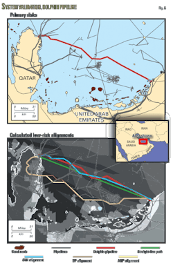
Fig. 5 shows the Dolphin pipeline. Brought online in 2007 at a cost of $3.5 billion, it is a 364-km marine pipeline delivering gas from Qatar's North field to the United Arab Emirates (OGJ Online, Mar. 8, 2007). The principal risks for this region are coral reef areas, areas of dense pipeline infrastructure, a high likelihood of excessive crossings, moderate commercial shipping activity, and a low seismic hazard along the eastern pipeline segment.
Fig. 5 also shows the analyses to have produced varying results, with the SWI alignment most closely following the actual pipeline route, its emphasis on land-based risks quickly directing it offshore. Its following breaks in the dominant commercial shipping layer leads to any local variations in direction.
The BP and AHP alignments are nearly identical, running southward along the axis of Qatar before turning east to complete a route far to the south of the actual pipeline. The BP and AHP methods' identification of the shore as riskier than surrounding land and sea influenced this path.
To avoid this risk, the two pipelines ran west and south through a low-risk area in Qatar, then out to sea between coral reefs along a path following the southern extent of a moderate-risk shipping corridor.
Table 3, the summary statistics table, shows the BP and AHP alignments as equally representing the lowest-risk path for the Dolphin pipeline. They are, however, more than 100 km longer than the SWI alignment and actual pipeline, resulting in a large project cost increase if built.
This result does not invalidate the method, however, as the lowest-risk path can emphasize intangible risks over cost risks. These two alignments show if the priority is to avoid risk, the best alignments will pass south of moderate commercial shipping risk areas.
In both examples, the SWI alignment produced the shortest of the low-risk paths, while the lowest-risk path was consistently produced by one or both of the pair-based methods. In both examples, at least one of the three weighting methods resulted in a close approximation of the actual pipeline route, and one of the three methods produced a suitable and economically viable alternative, demonstrating the importance of generating multiple solutions.
Several key risks, however, including political risks, were dropped from analysis due to a lack of data more detailed than the country's overall risk level. Digitizing some datasets from coarse resolution images made them not as accurate as other data.
Much of the data collected for analysis were also discrete rather than continuous, resulting in unnaturally sharp transitions between risk zones. In some cases, the calculated route appeared to come too close to developed oil fields, suggesting a need to reevaluate some minimum safe distance buffers. Finally, problems associated with the surveys (low sample size and survey fatigue) may have reduced the accuracy of calculated weights.
References
1. Overfield, R.E., and Collins, J.F., "Quantitative Risk Assessment as a Design Tool—Recent FPSO Experience," SPE Production and Facilities, Vol. 17, No. 2, pp. 72-77, 2002.
2. Dey, P.K., Ogunlana, S.O., Gupta, S.S., and Tabucanon, M.T., "A Risk-Based Maintenance Model for Cross-Country Pipelines," Cost Engineering, Vol. 40, No. 4, pp. 24-31, 1998.
3. Braestrup, M.W. (Ed.), Design and Installation of Marine Pipelines, Oxford: Blackwell Publishing Ltd., 2005.
4. Dey, P.K., "Integrated Approach to Project Feasibility Analysis: A Case Study," Impact Assessment and Project Appraisal, Vol. 19, No. 3, pp. 235-245, 2001.
5. Guo, B., Song, S., Chacko, J., and Ghalambor, A., Offshore Pipelines, Oxford: Elsevier, 2005.
6. Brown, T.C., and Peterson, G.L., An Enquiry into the Method of Paired Comparison: Reliability; Scaling; and Thurstone's Law of Comparative Judgment, Fort Collins, Colo.: US Forest Service, 2009.
7. Saaty T.L., The Analytical Hierarchy Process, New York: McGraw-Hill, 1980.
8. Berry, J. K., "Applying AHP in Weighting GIS Model Criteria," http://www.innovativegis.com/basis/Supplements/BM_Sep_03/T39_3_AHPsupplement.htm, 2003.
The author
More Oil & Gas Journal Current Issue Articles
More Oil & Gas Journal Archives Issue Articles
View Oil and Gas Articles on PennEnergy.com


