Consortium developing DRA model, algorithm
Assessment of Energy Saving in Oil Pipelines (AESOP) is in the process of developing the techniques required to use drag-reducer additives (DRAs) in pipelines, reducing energy consumption and increasing transport capabilities. This article focuses on the development of a DRA efficiency and degradation model and the description of an algorithm for optimal operation of pipelines using DRA
Drag-reducing additives
Oil companies seek to increase efficiency and transport capabilities. The best solution, when possible, is to increase the capabilities of the existing pipeline network, as other solutions such as increasing the truck fleet or building new oil pipelines require major capital investment and face sometimes major structural hurdles (highway crowding, environmental impact, etc.).
It has been shown that frictional pressure drops or drags, limiting the throughput of oil pipelines, can be significantly reduced by injection of long-chain polymers as DRAs. Despite extensive research in drag reduction over the past 4 decades, there is no universally accepted model that explains its mechanism.
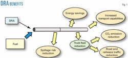
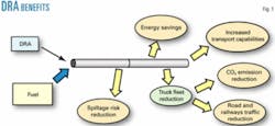
Fig. 1 shows the practical benefits of drag reduction. At the same pressure drop, the fluid moves at a faster flow rate, or the pipeline can maintain a constant flow rate even though the pressure drop is lowered.
One of the most important facts of polymeric drag reduction is that it only occurs in turbulent flow. Polymers change the flow characteristics of turbulent fluids by decreasing the intensity of turbulence. Drag-reducing systems show less turbulence in the core of the pipe. Drag-reducing polymers, however, do not directly affect the turbulent core but interfere with the bursting process, preventing the turbulence from been formed.
Not all polymers are equally effective drag reducers. Drag reduction is influenced by polymer solubility, polymer flexibility, polymer molecular weight, and solution relaxation time.
Another characteristic of drag-reduction systems is that they approach a maximum drag-reduction asymptote.
DRAs were first used in commercial pipeline operations in 1979. Gel-type DRA produced flow increases of up to 30%. A new generation of polymer-based liquid DRAs has been developed producing flow increases of up to 100%, while maintaining base product specifications.
As frictional pressure drop decreases, less energy is required to move the oil through the pipeline. So throughput can be maintained with reduced energy consumption or throughput can be increased without raising operating pressure.
It is well known that DRAs become less effective with the distance travelled by the base product in the pipeline and will also be degraded by passage through pumps, valves, and other equipment in the pipeline, and by temperature.
In spite of some very promising laboratory and small-scale field experiences in oil pipelines, there are still many open questions about how to apply new DRA effectively in complex and large installations. This technology has not been developed because of a lack of ability to design and operate the necessary installations.
The main focus of AESOP-which is partially supported by the Energy, Environment and Sustainable Development Program of the European Union’s Fifth Framework-is to develop the necessary techniques to allow large-scale industrial use of modern long-chain polymer DRA in order to reduce the energy needed to operate oil pipelines.
This focus can be divided into the following:
• Carrying out a systematic set of experiments in industrial pipelines to assess DRA efficiency, degradation, influence on measurement equipment, and effect on the quality of the base product and car engines when high concentrations are used.
• Developing computer models of polymer effectiveness and polymer degradation.
• Developing algorithms and computer packages for reducing the energy used, increasing productivity by reducing operating costs, and increasing transportation capabilities.
AESOP consists of Compañía Logística de Hidrocarburos SA (CLH), Madrid; Société du Pipeline Méditeranée Rhône (SPMR), Neully-sur-Seine, France; Société des Transports Pétroliers par Pipelines (TRAPIL), Paris; Energy Solutions Inc. (ESI), Copenhagen; the Andalusian Association for Research and Industrial Cooperation (AICIA), Seville, Spain; Fiat Research Centre (CRF), Trento, Italy; and Centre Spatial de Liege (CSL), Université de Liège, Belgium.
This article describes the main results obtained by the System Engineering and Automation Department of Seville University (AICIA)
The modeling
Efficiency and degradation models relate how the effective drag degrades along the pipes as a function of operating parameters such as initial polymer concentration, product, pipeline diameter, flow, and distance traveled. The models have been obtained by fitting a parametric structure to experimental data.
Two different types of models have been used:
• Modifications to pressure-drop equations (Colebrook or Hazen-Williams) to include the effect of the polymers and the introduction of a value of equivalent concentration of DRA, instead of the initial (injected) concentration, to model the degradation effect. This model is the analytical model.
• A neural networks model, training a neural network in a supervised manner using the data set collected in experiments. This is the neural model.
Experimental data
The data set used to fit and validate the models corresponds to field experiments performed by CLH and TRAPIL in their pipelines. Product was pumped for 5 to 10 hr through a pipeline section, with 0 to 25 ppm of DRA injected at the origin. Pressure, flow, temperature, and other variables are measured at intermediate points. The raw data are later used to determine the friction reduction achieved.
Data generated include: pressure and temperature at the pipeline entry point, middle points, and its end point; flow, density and viscosity values at the head of each pipeline piece; and the concentration of additive at various points along the line. More than 700 experiments have used the data.
Analytical model
The analytical model considers the efficiency of the additive with an experimentally adjusted mathematical expression and also models the degradation effect as a reduction of the effective DRA concentration.
A fixed-structure mathematical equation has been used to model efficiency. The formula computes friction reduction (%FR) when using DRA. Parameters are then adjusted to fit the experimental data. The main features of the formulas are:
• The value of friction reduction when no additive is injected is 0.
• %FR grows with the quantity of additive.
• %FR grows faster with little additive and there appears to be a saturation effect.
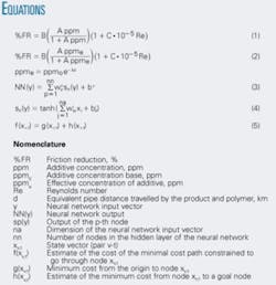
After considering different alternatives, efficiency has been modelled as a function of the additive concentration and the Reynolds number. The effect of other variables, such as type of product (gasoline or diesel) is included in the equation parameters to be adjusted with experimental data. Equation 1 is the proposed equation, where A, B and C are parameters.
It is generally assumed that the friction-reduction property of some polymers is lessened when the product with DRA travels along a pipe and passes through pipeline equipment. The effective concentration is obtained as a function of the travelled distance. Also, in order to consider the degradation due to passage through such elements as bends, valves, etc, an experimentally computed equivalent distance is used.
Equation 1 thereby transforms into Equation 2. Parameters A, B, C, and λ are obtained fitting the model to data. Table 1 shows typical values.
The distance between pumping stations in European pipelines is normally less than 200 km. For this reason degradation should be small. Equipment, valves, bends, and other discontinuities in the pipe, however, cause very strong localized degradation.
The quality of the model has been measured by the root mean square error (RMS).
If parameters are adjusted for a specific pipeline, the error in experimental data is around 2. (It is impossible to obtain more accurate results because of the measuring equipment.) If parameters are adjusted for a set of pipelines to obtain global values, the maximum RMS error obtained is 8.7.
Neural model
Models based on first principles are difficult to obtain due to the complex nature of the nonlinear partial differential equations of fluid motion. For this reason a black-box approach seems appropriate. Neural networks are known to be universal approximators.1 If a mapping exists among some independent variables and the FR, it is possible to construct a neural network that approximates such mapping, provided that sufficient information is supplied for training.2
This model would have the structure FR = f(y), where y is a vector containing the independent variables of the model to be chosen.
Training a neural network consists of adjusting the internal parameters of the net (weights) in such a way that its output NN(y) is close to f(y) for a set of observed values of FR and y.
An artificial neural network with one hidden layer computes a nonlinear function of its input vector y. This function is expressed in Equations 3 and 4. Coefficients wop, wipj, bo, and bip are the adjustable parameters of the network and are referred to as weights. Fig. 2 shows a diagram of the neural network described above.
In order to obtain a neural model, the available data have been split into two separate groups: the training set (TS) and the validation set (VS). The latter is used to avoid overtraining. Just 60% of all observations are used in training, with the rest going to the VS.
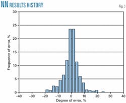
The same variables used in the analytical model were selected as the input vector: DRA concentration, Reynolds number, and equivalent distance. Different net sizes and training cycles were tried, with an error of about 6% being the best result obtained for a network with just three nodes in the hidden layer.
Fig. 3 presents the histogram of the error for that network.
The core of the software for optimal operation is an algorithm based on Bellman’s optimality principle. Evolution of pipeline states is computed with a specific steady-state pipeline model and simulator.
Pipeline model
The pipeline model used in this article is a hybrid dynamic model, driven by events and with a continuous behavior between events. The optimization algorithm uses events to set control variables.
Given a pumping sequence and an initial state, the model should be able to calculate the state of the pipeline at any given moment, the arrival time of the different batches, and the evolution of the level of deposits at terminal points.
This model is valid for networks with just one entrance point for the product (tree topology).
The topology of a pipeline network is defined by its component parts (Fig. 4).
As well as modeling of the physical characteristics of the pipeline, external effects which influence the behavior of the pipeline must be included.
The evolution of the pipeline will be driven by events. That is, the simulation algorithm will detect the events, and the evolution between states will be calculated by hydraulic equations. The events will be used by the optimization algorithm to adjust the control variables. The main events are:
• Arrival of interfaces at components; used normally to change the position of valves or to adjust the DRA injection pumps.
• Tank level reaching its limits; a constraint of the problem.
• Electrical tariffs changing; impacting connection and disconnection of the pumps.
Optimization algorithm
Some results exist for optimization of pipelines but only with monofluid systems.3
The proposed algorithm determines how to set the different pumps, valves, and DRA injection points at each interval so that the batch sequence is pumped in a desired period of time; optimizing use of electricity and DRA.
The control variables in the pipeline will be the status (on/off) of each pump, the position of the valves, the flow at the head of the pipeline (maximum pressure valves) and the DRA injected (ppm).
Some assumptions are made to simplify the problem.
First, it will be considered that the system operates in stripping mode. That is, each output node is working with an input flow proportional to the amount of product that the terminal has to receive from the current batch. This method of operating is widely considered the best way of using a pipeline. Notice that in stripping mode, the position of terminal and bifurcation valves depends on the batch passing at any given moment.
Second, by looking at typical characteristics of pump power consumption-flow, it is clear that the power consumption of the pumps grows slowly with the flow and depends mainly on whether the pump is connected. From the power optimization point of view, therefore, the best results will be obtained with maximum flow.
Finally, the accuracy of the dosage of DRA injection pumps is considered to be low. From a practical point of view, only discrete values of DRA injection will be considered. Typical values used in real pipelines are 0, 5, 10, 15, 20, and 25 ppm. Also, the concentration will be held the same for a whole batch.
Reducing the control variables to the on/off status of each pump and the DRA content of each batch, the problem can be stated as follows:
Given a batch sequence and a target time (maximum time to pump the complete batch sequence), the DRA concentration to be injected into each batch and the pump settings needed to minimize operational costs can be determined.
Current prices of DRA relative to electricity make it possible to approach the problem practically. It is more economic to connect electrical pumps than inject DRA, even at low concentrations. DRA is only used when pump configuration given maximum flow is unable to satisfy the time constraint. When it is necessary to inject DRA, the maximum flow configuration is normally used.
The algorithm determines if it is necessary to use DRA and computes the amount to be injected to minimize its consumption. Otherwise, it will optimize pump electricity costs.
DRA
A simulation of the complete batch sequence is computed, first considering no additive injection (0 ppm) in any batch or at any injection point. If the total simulation time is smaller than the target time, it is unnecessary to use DRA.
The algorithm to set the pumps optimally (described in the next section) must instead be used.
The second simulation uses 25 ppm in all batches. If the simulation time is larger than the target time, then it is impossible to verify time constraint. This simulation is performed at maximum flow.
In any other situation, the following DRA injection optimization algorithm is needed.
Now, the problem consists of determining the DRA injection for each batch. The decision must be made when a batch arrives at the injection pump (decision event) and the injection will be maintained for the entire batch. Usually, there is one DRA injection point at the output of each pipeline pump station.
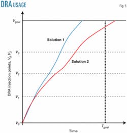
When operating in stripping mode, the position of the batches along the pipeline only depends on the amount of product that has been pumped (V). The batch position can, therefore, be shown by the pair (V,t).
The evolution of the system can be represented in the plane V-t and a trajectory from (0,0) to (Vgoal,tgoal) must be obtained. This way, decision events occur in the same order (same V), independently of the DRA injected to previous batches.
Obviously, time (t) depends on previous decisions (flows are going to be higher if batches inside the pipeline have been injected with high DRA concentrations).
Fig. 5 shows the plane (V,t) with two different trajectories (different DRA injections). Trajectory 1 uses higher flows because the DRA injections at the decision points were higher. This solution satisfies the time constraint. Trajectory 2 needed a smaller amount of DRA, but the obtained flows were unable to pump the batch sequence within target time.
The algorithm is based on a best-first- search algorithm. This method produces a search tree on which nodes represent the state of the system (the pipeline) at decision points. The root node is the initial state and successors of a node are the states reached when a decision action is applied.
Obtaining the successors of a node is called node expansion.
The objective is to reach a goal node connected to the root through the search tree.
Fig. 6 shows the tree inside the V-t plane, with higher flows (higher slopes) obtained via higher doses. Also, flows for the same injection are different at Decision Points 1 and 2, even when the batch’s situation is exactly the same. This is because the flow in V1 depends on the DRA injected in the V0-V1 interval.
A pipeline state is the position of the batches and is represented by the pair (V,t). The decision variable is the dose injected to each batch at every injection point. Every node has six successors (0, 5, 10, 15, 20, and 25 ppm.). A node represents the state of the pipeline when a new batch is going to arrive at an injection point and the child of that node is the state of the pipeline when the next decision point is reached (pumped volume).
All the successors of a node have the same pipeline state but different DRA consumption and pumping time.
The main problem with these algorithms is the combinatorial explosion when nodes are expanded. A best-search algorithm tries heuristically to reduce the number of expended nodes using an evaluation function, such that the node to be expended at any time is the one with the lowest evaluation function value. The optimization algorithm uses the cost function in Equation 5, in which the cost of this function is the volume of DRA injected.
The function g(xv,t) is computed easily during the search tree construction. It is the volume of DRA added from the beginning to state xv,t The heuristic function h(xv,t) is more difficult to estimate. This function must be as accurate as possible because the number of expanded nodes depends on this function.4
Electrical cost
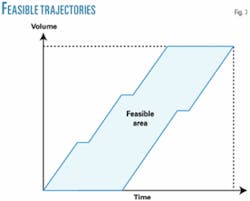
The state of the pipeline can, therefore, be shown by the pair (V,t), and the optimum control problem consists of determining an optimum trajectory in the plane V-t from point (0,0) to (target-volume, target-time).
The feasible trajectories are constrained by two curves (Fig. 7). The upper one is the curve resulting when pumping the batch sequence with the maximum capabilities of the system. Notice the horizontal pieces of the curve corresponding to intervals where the pumps have to stop either to avoid tank overflow or to permit maintenance. The lower curve is computed taking into account the minimum amount pumped in order to satisfy system needs. Notice the importance in that curve of tank overflows.
The electrical cost optimization algorithm uses a function with similar structure to the one used in the previous section (Equation 5), but its values are obtained in a completely different way. This optimization algorithm works in two steps. First, the function h(xv,t) is computed on a grid using Bellman’s optimality principle5 and, second, this function is applied to an accurate simulation of the transportation system.
Results
The algorithms presented here have been tested on a model of a real pipeline. It is a 300-km line, with four terminal points, two pump stations (one at the point of origin and one 90 km downsteam) and two DRA injection points, one at the output of each pump station. Three different electricity prices were used.
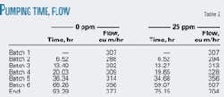
A batch sequence of six batches of different products with a total volume of 31,000 cu m has been simulated. Table 2 shows the pumping time and the flow obtained with the simulator at the beginning of each batch with two different additive concentrations, 0 and 25 ppm.
Table 3 shows the results for different goal times. Notice the sharp growth in cost when the goal time must be reduced.
Special consideration must be given to the last batches of a given sequence. At the end of the pumping, they are still inside the pipeline and affect the next batch sequence to be pumped.
When target time is bigger than 93.29 hr (Table 2), the second algorithm can be used.
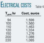
Table 4 shows electrical costs for different target times bigger than 94 hr when no additive is injected.
Acknowledgment
The authors acknowledge all the staff of AICIA and CLH involved in the AESOP project and the collaboration of the AESOP partners: SPMR, TRAPIL, ESI, CRF, and CSL.✦
References
1. Hornik, K., Stinchcombe, M., and White, H., “Multilayer feedforward networks are universal approximators,” Neural Networks, Vol. 2 (1989), No. 5, pp. 350-366.
2. Yuan, J.L., and T.L. Fine., “Neural-neworks design for small training sets of high dimension,” IEEE Transactions on Neural Networks, Vol. 9, (1998), pp. 266-280.
3. Van Zyl, J.E., Savic, D.A., and Walters, G.A., “A Hybrid Method for Operational Optimization of Water Distribution Systems,” Water Software Systems: Theory and Applications, Vol. 2, Ulanicki, B., Coulbeck, B., and Rance, J.P. (eds.) Baldock, Hertfordshire, England: Research Studies Press, 2001, pp. 89-97.
4. Ridao M.A., “Optimal use of DRA in oil pipelines,” Proc. IEEE System, Man and Cybernetics ’04, The Hague, , Oct. 10-13, 2004.
5. Bellman, R.E., and Dreyfus, S.E., “Applied Dynamic Programming,” Princeton, NJ: Princeton University Press, 1962.
