LOUISIANA HAYNESVILLE SHALE—3 (Conclusion): Operating envelope of Haynesville shale wells' profitability described
Mark J. Kaiser
Yunke Yu
Louisiana State University
Baton Rouge
The purpose of this third and final article is to characterize the operating envelope under which Haynesville shale wells are economic and describe the profit space through generalized net present value functional relations.
The two defining characteristics of Haynesville shale gas development are the high costs of drilling and completion and the high degree of uncertainty surrounding physical and economic parameters that affect project returns.
The significant and pervasive uncertainty surrounding many of the key play attributes has considerable impact on the economic merit of projects.
Adverse conditions in completion strategy or unanticipated physical characteristics of the geologic structure may arise. Regulatory events, such as restrictions on water use, disposal or fracture technology, can increase costs or cause operations to cease. Market events, such as low commodity prices, or higher than expected costs, can make projects unprofitable.
The key exercise in any economic analysis is the investigation of model sensitivities and the determination of the primary factors. By assigning probability distributions to the engineering elements of production, investments, and expenses, distributions of economic indicators are calculated and provide an assessment of project risk and return.
We utilize a design space approach to represent the uncertainty of the model parameters for expected future business environments. Net present value functionals are constructed that provide a measure of expected profitability conditioned on the values of the input data. Both before and after-tax assessment are presented to gain insight into the sensitivity and constraints associated with play economics.
Simulation
Simulation allows the user to include a large number of variables in a single model that can be rapidly built and analyzed.
The basis of most simulators is the Monte Carlo method that operates by selecting values from input distributions and combining them to determine an output distribution.
Simulating the economic performance of Haynesville wells allows us to:
• Understand how multiple factors interact with the profit metric.
• Understand the relative importance of each model variable.
• Capture the profit distribution and the range and likelihood of value.
The distribution shows the range of possible outcomes along with their frequency, which indicates the relative probability of occurrence. The probability weighted average of all occurrences is the mean of the distribution, or the expected outcome.
The expected range of each variable and the correlative structure between variables, if any, is an important element in modeling and determining appropriate ranges and correlations is key to accurate results. The exact form of parameter distributions is often less important than including all the relevant variables within their expected ranges.
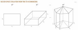
Design space
For two variables (x1, x2) assumed to follow uniform distributions, the net present value function NPV(x1, x2) is computed for each combination of x1 and x2 over a rectangular range, and with three variables, NPV(x1, x2, x3) is computed within a cubical region (Fig. 1).
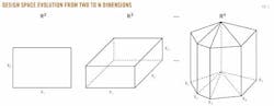
With n variables (x1, …, xn), the design space transforms into a hypercube and NPV(x1, …, xn) is an n-dimensional functional.
The design space represents the size and shape of the model parameters. If the parameters are expected to follow specific distributions, these can be applied, or if there are no a priori expectations, it is often convenient to assume uniform distributions.
The shape and size of the design space is a primary factor in determining the model output as illustrated in Fig. 2.
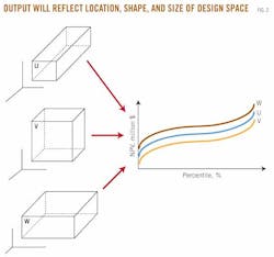
As the design space changes its position relative to the origin and as its shape and size changes, differences will be induced in the output metrics. If the decision-maker is confident the design space is representative of the investment opportunity, the distribution of NPV provides key information for a probabilistic assessment.
The mean of the NPV, E(NPV), is the expected outcome and standard deviation provides bounds on the expected uncertainty which enables us to look at both the probability and cost of failure as well as the expected gain.
NPV functional
The net present value functional is hypothesized as a linear function of the design variables:
where the parameters are sampled according to their distribution and the model coefficients are assessed by ordinary least squares.
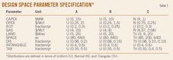
Three design spaces are specified in Table 1. Design space A was employed in the two-factor model in Part 2 of this series (OGJ, Jan. 9, 2012, p. 70).
Design space B truncates the variable ranges across the high-end of the distribution. Capital expenditures, for example, range between $5 million and $10 million in design space B rather than the $5-15 million range in design space A. Intervals on operating expense, gas price, royalty rate, and discount rate are also truncated. Since all of these factors, except gas price, represent a cost of business, design space B will lead to more favorable economics compared with design space A.
Design space C is described with probability distributions suggested by empirical analysis. Capital expenditures, for example, are described by the normal distribution with mean $9 million and standard deviation $1 million, so with 95% confidence the model attests that CAPEX will range between $7 million and $11 million. Operating cost and gas price are also assumed to be normally distributed. Triangular distributions are used for land, spacing requirements, discount rate, and corporate tax.
Model results
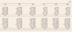
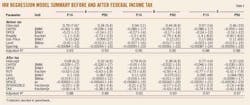
Model results are shown in Table 2 before and after-tax for design spaces A, B, and C. In Table 3, the pre and post-tax IRR models are calculated for P10 and P50 profiles.
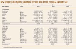
All the coefficients are of the expected sign and statistically significant except the discount and royalty rates, which are not always statistically significant or of the correct sign. Application of the NPV functional is straightforward and left to the reader.
Here we only comment on the value of the model coefficients via play economics. Consider the P50 before-tax model results for design space A. For each $1 million increase in drilling cost, NPV will decrease by $0.93 million, while a $1/Mcf increase in lifecycle operating expense will decrease NPV by $2.4 milion.
Royalty and discount rate yield similar results. A 1% point increase in the royalty rate, for example, is worth about $9.8 million, while increasing the discount rate by 1% point will erode NPV by $6.5 million. For a $1/Mcf increase in gas price, project value increases by $1.9 million.
The coefficients of the after-tax model cannot be directly compared with the before-tax case because the design spaces are structurally different and have different dimensions. The expensed items and amortized capital expenditures are only used to offset tax liabilities generated by project revenues.
For P50 production and design space A, a $1 million increase in capital expenditures will decrease NPV by $0.8 million, while a $1/Mcf increase in operating expenses will decrease NPV by $1.3 million. A 1% increase in the royalty and tax rate impact project value by $14 million and $4 million, respectively. As the tangible portion of capital expenditures increase, the operator is forced to depreciate more investment over the 5-year time period, which will negatively impact economics. The discount rate does not exhibit the appropriate sign, but it is also not significant, so it is not considered further.
NPV cumulative distribution
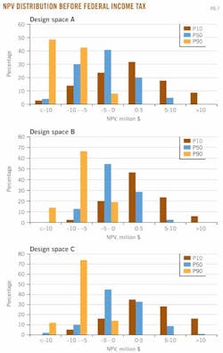
The cumulative distribution of NPV for a 100-iteration simulation is shown in Fig. 3 by production class and design space before federal income tax.
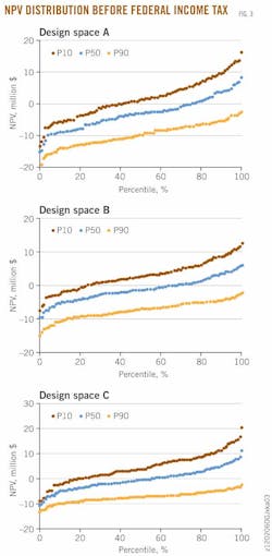
In design space A, about 60% of P10 wells and 25% of P50 wells are profitable, while in design space B, about 75% of P10 wells and 30% of P50 wells are profitable. In design space C, over 80% of P10 wells and 50% of P50 wells are profitable. P90 wells are not profitable under any scenario.
The explicit treatment of uncertainty provides a richness of information that has a number of advantages in decision making. The power of the probabilistic approach is that is provides a quantitative indicator of the probability and magnitude of loss. The probability of incurring a negative NPV for Haynesville wells is real and significant.
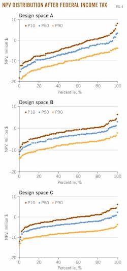
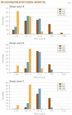
In Fig. 4, the after-tax analysis is depicted. Here, only about 25% of P10 wells and 5% of P50 wells are profitable under design space A; 30% of P10 wells and 10% of P50 wells are profitable under design space B; and 40% of P10 wells and 10% of P50 wells are profitable under design space C. P90 wells are unlikely to return their investment under most conditions.
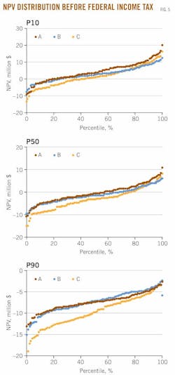
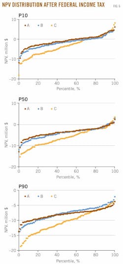
In Figs. 5 and 6, the NPV distribution by design space per production class illustrates the sensitivity of the model results.
For P10 wells, the before-tax model output is broadly consistent across the three design spaces, while for P50 and P90 wells, there is greater variation in the distribution.
In the after-tax analysis, the differences in the distribution curve across each design space are more significant. For high producing wells, the model results indicate robust profitability profiles that are relatively invariant with respect to the design space, while for average and marginal producers, the choice of design space has a more significant impact on profitability.
NPV histogram
NPV histograms are depicted in Figs. 7 and 8, and expected value and standard deviation are depicted in Table 4.
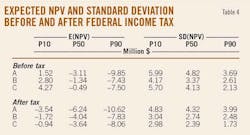
In design space A, P10 wells before-tax realize E(NPV, P10) = $1.52 million while for P50 wells, E(NPV, P50) = –$3.11 million. On average, the high performing well will create value under the design parameters specified in A, while the average well will not be profitable. Standard deviations are large reflecting the size and shape distribution of the design space.
In design space B, the expected values for each production class improve as expected: E(NPV, P10) = $2.8 million and E(NPV, P50) = –$1.34 million. The P50 well still does not create value. Design space B yields better economic metrics and result in a lower standard deviation than design space A because B is smaller and positioned more favorably within the profit space.
In design space C, E(NPV, P10) = $4.3 million and E(NPV, P50) = –$0.5 million. Profitability depends on production performance, gas price, costs, tax rates, and incentives.
If the decision-maker believes design space B and C are accurate representations of the available investment, then the decision to invest will likely be based on the expected initial production rate.
P10 wells generate value, but P50 wells do not, so unless the operator believes the well will come in as a P10 producer, investment decisions will likely be delayed unless the operator enjoys significant cost advantages or needs to drill to hold acreage.
More Oil & Gas Journal Current Issue Articles
More Oil & Gas Journal Archives Issue Articles
View Oil and Gas Articles on PennEnergy.com