COMMENT: The importance of dependencies in multireservoir prospect evaluation

Editor's note: This article comments on "Dependent on dependence: Are economic calculations of expected hydrocarbon accumulations worthwhile?," by J.A. MacKay and Ian Lerche, OGJ, Nov. 7, 2011, p. 56.

Timothy Nieman
Decision Applications Inc.
Saint Helena, Calif.

In the opening paragraphs of the above article on dependencies between two reservoirs, the authors state that: "In particular, varying the allowed probability for the dependent reservoir is shown to not influence either the expected project value or the standard deviation around the expected value. The result is that the cumulative probability of obtaining a hydrocarbon reserve in excess of a fixed amount is also not influenced by the dependence probability chosen and behaves as though the two reservoirs were totally independent of each other."

If true, this would be a rather striking conclusion; that the distribution of reserves for a multireservoir prospect does not vary as the strength of dependencies between the reservoirs varies. However, this is not true.

In multireservoir prospects, the practice of focusing on understanding the nature of the dependencies is commonly done for the very reason that it ensures the evaluation of the combined opportunity is done properly. The authors here state that it doesn't matter because they claim the standard deviation does not change with different assumptions about the dependency. But it can be easily shown that the standard deviation does change.

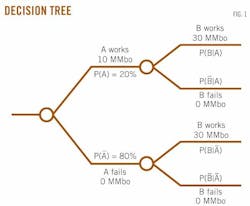
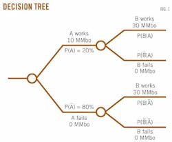
First, let's examine the case described by the authors where there are two reservoirs involved. In their example, the authors describe the following situation. Reservoir A has a 20% probability of success with reserves of 10 million bbl in the success case. Reservoir B has a 10% probability of success with reserves of 30 million bbl in the success case. The authors calculate the expected value (5 million bbl) and standard deviation (which they incorrectly state as 9.2 million bbl) for the case where the two reservoirs are independent (that is, where P(B|A) = P(B|notA) = 10%). The decision tree for this scenario is shown in Fig. 1.

They then identify a set of feasible values for P(B|A) that preserve the total probability of success for reservoir B at 10% (P(B|A) can range from 0 to 50%), and state that "the standard deviation around the expected value is also independent of the value chosen for Pc within the limiting range and is 9.2 million bbl, in agreement with the situation where A and B are taken to be independent when the standard deviation is also 9.2 million bbl." Note here that Pc is P(B|A) in Fig. 1, the conditional probability of success for B given success in A.

Let's calculate variance and standard deviation for all feasible values for P(B|A). The variance of the total reserves as a sum of two variables is given by:

Var(X+Y) = Var(X) + Var(Y) + 2 * Cov(X,Y)

Where the equations for variance of one variable and covariance for discrete random variables are given, respectively, by:

Var(X) = E[(X–µ)²] = ∑iP(xi) (x–µ)²

Cov(X,Y) = E[(X–µ_x)(Y–µ_y)] =
∑_i,jP(x_iy_j) (x_i–µ_x)(y_j–µ_y)

We can already see from the equation of Var(X+Y) that the authors claim that the standard deviation (square root of variance) is invariant will only hold if the covariance is a constant under all assumptions about dependence. The covariance of independent random variables is zero; the covariance of dependent random variables is nonzero.

Returning to the example, for all cases we get:

Var(A) = 16 million bbl₂

Var(B) = 81 million bbl₂

For the independent case where P(B) = P(B|A) = 10%, we get:

Cov(A,B) = 0

Var(A+B) = 97 million bbl₂

Therefore the standard deviation for the independent case is 9.85 million bbl, not 9.2 million bbl, as stated by the authors.

We can repeat this calculation for all possible dependent cases. Table 1 shows the calculations done every 10% across the feasible range defined by the authors.

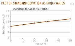
A plot of standard deviation as a function of P(B|A) gives the result shown in Fig. 2.

This relationship shown in Fig. 2 is consistent with typical behavior for multiple reservoirs; the more strongly positive the dependence, the greater is the standard deviation in the combined reserves forecast.

The bottom line here is that dependencies do matter in these types of multiple reservoir cases—the distribution of forecast reserves will change with your assessment of the strength of dependencies. And counter to another of the authors' conclusions, dependencies also affect the expected volatility in portfolio problems.

The authors' statement that we are left in a quandary is incorrect. It requires effort, expertise, and careful calculations, but we have methodologies for making rational estimates of the strength of dependencies and for assessing the distributions of reserves and economic values in both project and portfolio evaluations.

The author

Timothy Nieman ([email protected]) is the founder of Decision Applications Inc. in Saint Helena, Calif. He has 26 years of experience in the energy industry, including 16 years leading numerous projects involving application of decision and risk analysis methodologies, and 10 years as a petroleum geophysicist. He is also an active instructor of industry courses in petroleum economics, decision analysis, and quantitative modeling. He has a BS in geology and MS in geophysics from Michigan State University and an MBA from Rice University.

More Oil & Gas Journal Current Issue Articles
More Oil & Gas Journal Archives Issue Articles
View Oil and Gas Articles on PennEnergy.com