Managing Oil & Gas Companies: Probabilistic methods with simulation help predict timing, costs of projects
Continuous probabilistic techniques involving simulation can help managers predict the likelihood of time and cost overruns in all types and sizes of oil and gas projects.
By deriving time and cost forecasts from a series of trials, simulation offers insight into project risks and quantifies the chances that a project will be completed within budget targets and deadlines.
Unlike discrete deterministic methods, probabilistic simulation systematically incorporates the risks associated with a range of uncertainties about costs and completion times of project activities. The results take the form of a numerical distribution, with each value in the distribution linked to a probability of its occurrence. The distributions and their intermediate calculations can be used in a variety of ways to enhance project planning, evaluation, and decision-making.
Advances in personal computer processing capacities and versatile spreadsheet software make it possible for sophisticated simulation models to be built and applied efficiently to a wide range of projects. For a medium-size project-one with 20 activities performed in five parallel sequences involving complex dependencies-a model simulating costs and time and analyzing risks and critical paths can be constructed, run, and evaluated in a single working day.
As with deterministic methods, probabilistic techniques depend upon well-researched estimates for ranges of activity costs, times, and resource requirements as their basic input data.
The approach recommended here is to integrate deterministic and probabilistic models and run them in sequence.
Because a project is more than the sum of individual activities, a network approach is crucial to all deterministic and probabilistic techniques. Important questions to be answered are:
- When can the project as a whole be completed?
- Can it be delivered on time and within budget?
- What are the risks associated with achieving specific cost and time targets?
Deterministic methods used in isolation can provide answers to these questions. Probabilistic techniques improve the answers. However, simulations require rigorous completion of the deterministic calculations in order to develop valid models.
Critical path networks
To identify interdependencies between project activities, managers often use a deterministic technique known as critical path analysis.
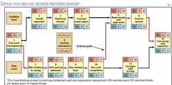
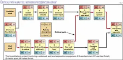
Critical path network diagrams quantify project priorities based on duration estimates for all activities. Fig. 1, the network diagram for a hypothetical project involving the drilling of a sidetrack well and installation of separation equipment, uses precedence diagram notation, which is common in project-management software. The block schematic basis of the notation allows for integration into spreadsheet workbooks.
Activities appear on the diagram as numbered blocks, each of which contains a duration estimate in its top middle cell. Arrows between blocks indicate sequence constraints and links between all project activities.
The first step in any network analysis is the "for ward pass." It involves the addition of activity durations in sequence along the arrows from left to right. If there is more than one possible path through a network, the duration totals depend on which path is followed. The earliest start (ES) time of an activity at any converging point in the network depends upon the earliest finish (EF) time of the latest of the activities feeding into it. The ES time of an activity appears in the top left cell of its block diagram. The EF appears in the top right cell.
The next step in critical path analysis, called "backward pass," is to calculate the latest permissible finish and start times for each activity.
The planner posts the earliest start time of the final activity (far right of the diagram) in the latest finish (LF) cell at the bottom right of blocks for activities feeding it-that is, those to its immediate left. He or she then calculates the latest start (LS) times of those activities by subtracting project durations from the LF numbers. The LS values appear in the lower left cells of the diagram blocks.
This subtraction process continues through the network from right to left. Where more than one possible path through the network exist, the latest ES of the subsequent activities (those to the right on the network) must be selected as the LF time for the immediately preceding activity.
The last cell to be filled in each activity block, the middle position of the lower row, indicates the amount of slack, or waiting time, potentially available between the activity's start and finish. Called "float," it is the difference between an activity's EF and LF.
Project network logic dictates that there be at least one sequence or chain of activities with float values of 0-that is, that EF and LF values be identical in each activity. This sequence is the critical path of activities, so called because it is critical to the successful completion of the project within the earliest possible time determined by the analysis. All activities are usually important, but the critical activities are those that should claim priority for resources and for management attention. By definition, the first and last activities of the network have zero float.
In reality, there is usually uncertainty associated with the duration of each activity. If the duration of each activity can vary between the limits set for uncertainty, the critical path through the network can also vary. Deterministic calculations take no account of this fact.
A probabilistic approach applies the same network logic but uses activity-duration distributions rather than single point values.
Probabilistic applications
After completing the network time analysis described above, the planner can apply probabilistic methods to allocate duration and cost estimates to each activity.
The estimates are selected at random for each simulation trial, based on a random number generator, from distributions defined for each activity. As iterations (trials) of the simulation are repeated, chance decides the values of the selected input variables within the limits of the distributions.
Different total project durations and total project costs will almost certainly result from each iteration. Computer processing speed is now so rapid that time and cost analysis of a project network can be repeated and recorded many hundreds of times very rapidly.
The planner executes many trials, in which equations formulated to combine logic relationships and sequences (for example, project networks) with numerical values of the components (for example, activity times and costs) are evaluated in each trial.
The frequently used Monte Carlo simulation technique produces a large sample of results that can be analyzed statistically to predict the most likely duration, completion date, and cost for any project activity.1 The activity that is usually of most interest from the timing perspective is the last project activity that gives the full project duration and completion date if linked to a specific project schedule.
Input variables are treated either as single-number estimates or probability distributions where uncertainty is involved. These variables may behave independently of each other or be related with complex dependencies. Project network and precedence diagrams reveal some dependencies between activities, but others are often more subtle and require careful consideration in defining the calculation algorithms.
Each simulation trial must perform critical path analysis if the total project duration is to be computed as a key output parameter, in addition to the sum of all the component activity durations. However, as different times will be sampled for each activity in each iteration of the simulation, the critical path may change for some iterations. Algorithms must be written that account for this, essentially performing a forward and backward pass for each iteration.
Random numbers between 0 and 1 are used to sample cumulative probability distributions of the input variables. The resulting values of the key dependent variables calculated by each trial form probability distributions that can be analyzed and presented statistically to yield information more useful than single-point (deterministic) outcomes.
Input distributions
In order to develop a probabilistic project model, the planner must first consider every project network activity and decide how much confidence can be placed in each time and cost estimate made for it.
Input variables are commonly described in terms of two or three points. For example: P10 (10th percentile, or 10% chance of being less than); measure of most likely occurrence or central tendency (mode or P50/median, values for which are not the same in skewed distributions), and P90 (90th percentile or 90% chance of being less than). These points are then transformed into mathematically specified cumulative probability distribution types-triangular, normal, lognormal, or uniform-for sampling in the simulation.2
In addition to mathematically defined distributions, some input data distributions can be defined by real historical data. These empirically defined distributions may or may not be similar to the mathematical distributions.
Historical performance of similar activities in recently completed projects is no guarantee that such activities can be performed to identical specifications in the future. Planners should therefore view historical data critically and usually extend the upper and lower limits of distributions to recognize other outcomes that might occur in the future.
In many cases, activity-cost distributions are constrained by commercial contractual terms. Some examples are fixed-price, gain-share, and profit-share contracts, where contractors assume significant risks of cost and time overruns in exchange for a share in any cost savings made relative to a target budget. Algorithms need to be written to customize sampling of such contractually and historically derived distributions.
The project manager should check how a simulation model defines and samples the distributions input by the planner. Although data may be input as three points, that does not mean the simulation defines or samples the data in a triangular form. Some algorithms sample distributions uniformly regardless of input.
Studying the input parameters as sampled by the simulation iterations (trials) to check for credibility is an important part of the analysis. Credibility, among other things, means that no unrealistic negative values are sampled by the simulation due to poorly defined input probability distribution.
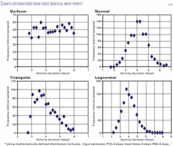
Fig. 2 illustrates how a three-point activity duration range is sampled as four different mathematical distributions to each provide a different set of values for that activity in the simulation trials.
During the preparation of simulation algorithms, the planner also must account for dependencies between activities in projects with more than one path of parallel activities. The dependencies will be evident in network and precedence diagrams.
The careful analysis essential to handling dependencies is beyond the scope of this article. What the planner must remember is that it is usually not realistic to assume that all activity cost and time distributions can be independently sampled by unrelated random numbers.
Output distributions
The calculated distributions resulting from a simulation can be displayed in a variety of ways to suit a range of objectives. Prior to detailed statistical analysis, frequency distributions help to reveal visually the shape of the distributions.
Sometimes it is useful to display such frequency distributions for both cost and time in conjunction with the provisional target objectives defined by the most likely deterministic estimates. It is also important to establish whether the output data are symmetrical or skewed.
The key information is unlocked from the output distributions by statistical analysis. The percentiles indicate the range of possible outcomes, and the arithmetic mean provides the best indicator of central tendency for most calculated distributions. A cumulative probability plot with mean and deterministic most-likely values superimposed on it is a very effective way of describing and illustrating a calculated distribution.
The shape of the frequency distributions can reveal whether the resulting distribution is well enough defined for meaningful statistical analysis. Choosing the number of iterations required to achieve statistical stability in the calculated simulation metrics is initially a trial and error process. It will vary from project to project depending upon the complexity of the network and the input distributions.
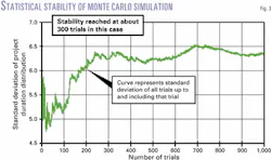
Calculating a running standard deviation of the results of all simulation iterations up to that point for a key output metric is a more useful way to assess statistical stability than visual inspection of the frequency distribution itself. As the simulation trials build up, a running standard deviation helps to identify when statistical stability has been achieved for the project being modeled.
Fig. 3 illustrates how such a running standard deviation typically illustrates that stability has been achieved. It is prudent to run the simulation for several hundred trials beyond initial stability. With modern computer power this is usually not a significant limitation to simulation speed.
Quantifying risk
One of the advantages of using simulation techniques and of defining project costs and durations as calculated distributions, as opposed to single-point deterministic calculations-is the ability to quantify uncertainty, risk, and opportunity.
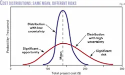
As used here, the term "uncertainty" means the magnitude of variation about a mean value in either a positive or negative direction. "Risk" is the magnitude of variation in a direction away from the mean that will have a detrimental impact on the project (higher cost, longer duration, or both). "Opportunity" is the magnitude of variation away from the mean that will have a favorable impact on the project (lower cost, shorter duration, or both).
Fig. 4 puts these terms into perspective by comparing two projects with identical mean total costs but different risk profiles.
Uncertainty associated with a distribution is commonly quantified with the standard deviation about its mean. But standard deviation becomes less meaningful for highly skewed distributions. And project managers are often more interested in measuring, monitoring, and mitigating risks than they are in broadly quantifying uncertainties or opportunities.
One simple measure of risk is the number of simulation iterations that produced results exceeding specified targets, expressed as a percentage of the total. This measure indicates the likelihood of a target's being exceeded but says little about the amount by which the target is missed.
A useful indicator of the magnitude of risk associated with exceeding targets is the semistandard deviation (SSD), the mean squared deviation of a distribution occurring above a target value. The SSD is calculated in the same units as the distribution.
Evaluating SSD for a range of potential project cost and duration targets can help planners set meaningful and achievable budget targets. SSD relationships also can help project managers focus on targets and monitor progress throughout the life of the project. They also can help planners establish realistic safety time buffers to be incorporated as contingencies in project schedules.
Actual project events are of course unlikely to exactly follow simulation forecasts. Attempting to quantify the range of possible outcomes and risks associated with them, however, is more useful than the deterministic alternative of evaluating a most-likely case and running high and low sensitivity cases.
The probabilistic method enables the possible range to be quantified in terms of its likelihood of occurrence and the risks of exceeding targets to also be identified and quantified.
Using such techniques in the planning and monitoring of projects helps managers make consistent decisions and remain aware of the magnitudes of risks involved.
References
- Wood, D.A., Applying Monte Carlo simulation to three-stage E&P risk analysis, in Three-stage approach proposed for managing risk in E&P portfolios, OGJ, Oct. 23, 2000, pp. 69-72.
- Murtha, J., Janusz, G., Spreadsheets generate reservoir uncertainty distributions, OGJ, Mar. 13, 1995, pp. 87-91.
This article is condensed and adapted from an Oil & Gas Journal Executive Report entitled Using Simulation to Improve Planning, Risk Assessment, and General Management of Oil and Gas Projects by David A. Wood. To order or for further information, call 1.800.752.9764, outside the US 1.918.831.9421, or send an e-mail to [email protected]. Please refer to Item No. OGJER13.
The author
David A. Wood is an exploration and production consultant specializing in the integration of technical and economic evaluation with management and acquisitions strategy. He is a director of E&P management courses with the College of Petroleum Studies (Oxford, UK). After receiving a PhD in geochemistry from Imperial College in London, Wood conducted deep sea drilling research and in the early 1980s worked with Phillips Petroleum Co. and Amoco Corp. on E&P projects in Africa and Europe. From 1987 to 1993 he managed several independent Canadian E&P companies (Lundin Group), working in South America, the Middle East, and the Far East. From 1993 to 1998, he acquired and managed a portfolio of onshore UK and North Sea companies and assets as managing director for Candecca Resources Ltd. Wood is the author of four Oil & Gas Journal Executive Reports. His e-mail address is [email protected].
