Program distributes rock properties for reservoir modeling

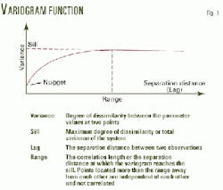
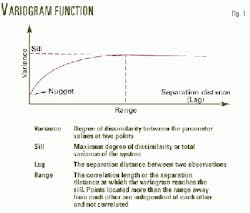
The variogram function (Fig. 1) at the heart of the statistical models relates the variance of a parameter to the separation distance between two measuring points (the lag). In reservoir modeling terms, petrophysical properties are spatially unpredictable when the correlation length or range of the property is less than the grid cell size.

Grid cells are typically at least tens or hundreds-of-meters on a side, so that, when the model expects a property to reach its maximum variance (sill) within meters from a measuring point, any single grid cell can take on any value within its sill.

One reasonable solution for such a case considers that the property is randomly distributed, taking on values within any grid cell that are within limits of its maximum variance. The process of randomly distributing petrophysical properties is essentially a process of conditional simulation with a range of zero, which is a specific class of stochastic modeling.

Petrophysical properties typically have short correlation lengths of a few meters or less in reservoirs where diagenetic processes have radically altered the original rock textures.

In carbonates, a well know fact is that dolomitization of an original lime mud matrix leads in some cases to formation of intercrystalline porosity, and leaching of corals, stromatoporoids, and other fossil constituents leads to formation of moldic pores.

In such systems, permeability depends on the juxtaposition of moldic pores and the presence of sucrosic intercrystalline porosity. Less common but equally important is formation of storage capacity through the dissolution of feldspars and other minerals in fractured granite reservoirs.

One cannot contour petrophysical properties over the inter-well distances in these types of carbonate and igneous reservoirs because they are related to the effects of diagenetic processes that are for all practical purposes trendless.

Carbonate reefs, in particular, are extremely variable in terms of primary facies and diagenetic modifications. Therefore, not surprisingly, many authors have stated that reservoir properties are difficult or impossible to correlate between wells in reef structures.^3-5

In 1979, Mungan concluded while modeling a Canadian Pembina Nisku reef reservoir that no layering was present and that a random distribution of rock properties would be appropriate.³ Accordingly, he used a table of random numbers and manually assigned rock properties to each of 360 grid cells in his reservoir model.

Mungan's approach was insightful because, about 12 years later, Patel and Broomhall concluded on the basis of extensive horizontal well drilling in several Pembina Nisku reefs that these structures are even more heterogeneous than originally perceived.⁶

In 1983, Nagai used a layering approach to build a model of the West Texas Wolfcamp Reef, even though he concluded that reservoir features could not be correlated across the reef.⁵ He obtained interwell grid cells properties by simple interpolation.

To obtain a pressure history match, Nagai arbitrarily increased the degree of vertical communication in his layered model by an order of magnitude.

Dietrich, while modeling a carbonate reef reservoir in the Volga region of Russia during 1995, also concluded that it was not possible to match the pressure history with a deterministic layering approach. Missing was the high degree of inter-grid-cell communication necessary to match the very low pressure gradients measured throughout the reef.

This led him to use a revised approach similar to Mungan's approach involving manual random distribution of properties in each grid cell, followed by a successful match of historical reservoir performance.

The computer program (see Editor's note at the end of the article to obtain a free copy) was subsequently written to automate the random distribution process.

This program has been used to build models of a fractured granite reservoir in North Africa and a super-giant carbonate reservoir in the Middle East, where spatially unpredictable variations of rock properties caused by diagenetic effects warrant its application.

Stochastic modeling

One can use the computer program to develop a reservoir description by randomly distributing porosity and net-to-gross ratio (NTG) to each grid cell of a reservoir model without regard to spatial correlation. The porosity may then be used with user input porosity and permeability correlations to determine permeability in each grid cell, or alternatively the permeability may also be distributed randomly.

In addition, the user may assign relative permeability tables according to his own porosity ranges, thereby allowing a distribution of endpoint saturations (connate water and residual oil saturation data) as a function of porosity.

Finally, one may adjust vertical transmissibility on a cell-by-cell basis by entering a threshold grid cell NTG level into the program. This threshold is a level below which vertical communication is not allowed.

At the heart of the program are cumulative distribution functions (CDFs) for NTG ratio and porosity that a user prepares from core and log analysis data. The CDF uniquely defines all of the probabilistic properties of a random variable.¹

Given a random variable X, the cumulative distribution function F(x) is defined as F(x) = Prob(X < x), or in words F(x) is the probability of finding a value of a random variable X that is less than or equal to x.¹

The user prepares CDFs for each rock-fabric unit that may be of interest. One may define a rock-fabric unit as a package of reservoir rocks with similar petrophysical characteristics that appears in all or most of the wells.^{1 2} These are then sampled by a random number generator to populate the 3D rock-fabric domain or domains.

Each time the program executes, a new spatial distribution (realization) of rock properties is obtained. The user builds the property CDFs by using core and log analysis of all footage penetrated within a given rock-fabric unit. This process is similar to shale-size CDFs that are built on the basis of outcrop studies and are used for the stochastic modeling of shales.

As a final step in the procedure, the user over-reads the random property distributions at and near the wells using specific core and well log data to ensure consistency with the well control.

An ASCII text file contains the user generated initial data. The program outputs the generated properties to ASCII text files with keywords and a format that allow inserting the output directly into a simulator input data file.

Program output can be input into such reservoir simulators as Halliburton VIP and Schlumberger GeoQuest ECLIPSE. Building keywords are NETGRS (NTG), POR (PORO), KX (PERMX), ISAT (SATNUM), and MULTZ (MULTZ).

Carbonate reservoir example

The first example demonstrates the application of the program to a Lower Cretaceous carbonate shelf reservoir in the Middle East.

Carbonate rock-fabric flow units

The Middle East carbonate reservoir has two rock-fabric flow units: upper and lower. Impermeable mudstones separate the units.

Total porosity within each unit is controlled mainly by variations in grain size (primary porosity), bioclast content, the presence of argillaceous material, and subsequent exposure to shallow meteoric waters through sub-aerial emergence, and later burial diagenesis.

The contribution of primary inter-particle porosity and secondary intra-particle porosity varies in each unit with effective permeability controlled by pore size and degree of diagenesis.

Wackestones-packstones with thin grainstone-packstone bands dominate the upper unit that consists of oolitic, fossiliferous, and bioclastic limestones with various gastropods, echinoids and rudists, with selectively dolomitized intervals and micritized bioclasts.

The upper unit has good primary inter-particle porosity and some secondary intra-particle porosity, with occasional leaching and cementation of bioclasts. Minor selective dolomitization occurs and there is no evidence of extensive diagenesis by calcite or ferroan dolomite of the uppermost sequence that grades upward into finer grained, offshore slope and deeper marine shales, without sub-aerial emergence.

The lower unit has similar lithologies with local development of coarse packstone-grainstone bands. The upper boundary is an unconformity with reworked, oxidized pebble lags embedded in friable silt and marl that may indicate sub-aerial exposure.

The unit is interpreted to have a more restricted shallow marine to lagoon environment with higher argillaceous content with a general reduction in grain size.

Primary inter-particle porosity in the lower unit is less than in the upper, and although secondary intra-particle porosity occurs, the interval has poorer reservoir quality given the finer grain size, clay content, and effects of meteoric diagenesis related to the unconformity.

Carbonate log data

The reservoir model included a 3D-simulation grid system of about 75,000 grid cells that had 20, 5.25-m thick layers in the upper unit and 40, 6.875-m thick layers in the lower unit.

After the user develops blocks of continuous raw log data for total porosity and water saturation corresponded to these layers, calculations determined the average NTG ratio and total porosity for each layer or block in each well.

In this example, cutoffs of 4.5% porosity and 50% water saturation defined net pay.

Carbonate distribution

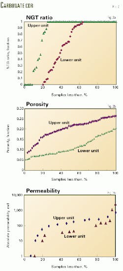
The next step prepared cumulative distribution functions for NTG ratio (Fig. 2a), total porosity (Fig. 2b), and permeability (Fig. 2c) for each rock-fabric unit by putting into order the calculated data.

The word "sample" in these CDFs refers to a calculated average property for a layer or block interval in a well.

The total number of samples for preparing each CDF is equal to the number of blocked intervals in all wells with available logs. CDFs for the upper unit reflect a much better rock quality than for the lower unit, as previously discussed.

The permeability was distributed randomly because cross-plots of total porosity and permeability showed no correlation. The permeability in this carbonate is principally a function of inter-connected leached stylolites and micromoldic pores formed after the dissolution or incomplete dissolution of skeletal grains. The micro-porosity, which is substantial, adds little to the permeability.

The lack of correlation is not surprising. In this type of system, one might expect a correlation between effective porosity and permeability, but not between total porosity and permeability.

Carbonate property distribution

The computer program used the CDFs, randomly sampled, to populate the reservoir model. It entered each CDF about either 25,000 or 50,000 times, depending on the number of grid cells used for each rock-fabric unit. This determined a property value for each grid cell.

A "realization" is a single random property distribution that results from this procedure.

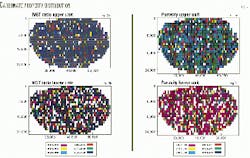
Fig. 3 shows plan views of a single realization for NTG ratio and total porosity. The white cells contain nonporous, nonpermeable rock, because their NTG ratios are zero or near zero. In the reservoir simulation, these white cells were not active and fluids were required to flow around them.

Although any given grid cell will be either active or inactive and take on different values for rock properties in different realizations, the frequency of occurrence of any given property value within the entire 3D domain will be exactly the same as shown by the CDFs.

In other words, although the distributions will differ with each realization, the statistical features of each distribution will remain unchanged.

This example found connate water saturation to be inversely related to total porosity. For this reason, connate water saturation was distributed on the basis of grid cell total porosity, not randomly.

A grid cell with a high total porosity was assigned a low connate water saturation and a cell with a low porosity was assigned a high connate water saturation.

The computer program defined and distributed four different rock types or porosity classes, each having unique endpoint saturations and relative permeability-capillary pressure functions.

Fractured granite basement example

Although fractured igneous reservoirs are uncommon, these reservoirs produce oil in California, Indonesia, Japan, North Africa,⁷ and offshore Viet Nam.⁸ The second example demonstrates the random distribution as applied to a large Pre-Cambrian fractured granite reservoir in North Africa.

Granite rock-fabric flow units

Based on log analysis and well productivity indices, the North African reservoir has three rock-fabric flow units: a basement relief unit, a western fractured basement unit, and an eastern fractured basement unit.

This reservoir is an example of a nonporous fractured reservoir in which the matrix is impermeable and contains no oil in place. Oil reserves and fluid flow are restricted to a network of open channels and connected vugs formed by aggressive waters flowing through the fracture system and dissolving portions of the matrix.

Secondary porosity can be well connected, forming a system that branches off the primary fracture network.

Even if one could possibly describe the primary fracture geometry, one could not reasonably approximate the pattern for the secondary porosity development.

In this example, the premise for the random distribution procedure is that rock properties are not predictable as a function of position in an igneous intrusive altered by diagenetic processes.

The best rock quality occurs within the basement relief unit and the eastern fractured basement unit. An unconformity occurs at the upper boundary of the basement relief unit, and the intensity of faulting is greater in the eastern portion of the reservoir.

Perhaps these are the reasons for more surface area to be exposed to the movement of meteoric waters in these rock-fabric units and, therefore, secondary porosity development is greater within these units.

Granite log data

The reservoir model included a 3D-simulation grid system of 45,000 grid cells that divided the overlying basement relief unit into 4 layers and the underlying western and eastern fractured basement units into 21 layers. Each layer was 15-m thick.

As in the carbonate example, the continuous raw log data for total porosity and water saturation were blocked to correspond to these layers and average NTG ratio and total porosity values were calculated for each layer or block in each well.

The granite reservoir model included a 2.3% total porosity and 60% water saturation cutoffs to define net pay, and used more than 4,500 m of well penetration data from numerous wells

Granite CDFs

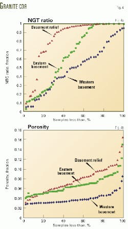
The next step prepared cumulative distribution functions for NTG ratio (Fig. 4a) and total porosity (Fig. 4b) for each rock-fabric unit by placing the calculated data in order.

Granite properties distribution

The computer program used the entered CDFs to generate NTG ratio, total porosity, and permeability distributions for the reservoir model. Fig. 5 shows the porosity distribution.

The program has distributed better rock quality to the basement relief unit over the entire upper portion of the reservoir and in the eastern fractured basement unit in accordance with the CDF features.

The spacing between the well-control points prevented the determination of a sharp interface between the western and eastern fractured basement units. Therefore, the program randomly assigns either one or the other of these rock-fabric units to the various grid cells representing a changeover zone that divided them.

In other words, the program as coded may be used to distribute randomly both petrophysical properties and rock-fabric units, if necessary.

Random distribution benefits

These examples show that random distribution of petrophysical properties, conditioned by data from cores and well-log analysis, provides highly heterogeneous models with good interconnectivity.

This type of model may be a better alternative than a deterministic model for describing complex carbonate and granitic basement reservoirs in which there is good pressure communication. Deterministic models, as built, almost invariably consist of some areally extensive low-permeability layers that will reduce the degree of vertical communication and introduce strong pressure gradients that may not be observed.

In the procedure described in this article, rock-fabric units are distributed deterministically and petrophysical properties are distributed randomly within each rock-fabric unit.

Where there is uncertainty concerning the position of the boundary separating two rock fabric units, one may define changeover zones between two units and within these zones the units may be randomly distributed.

Each curve in Figs. 2 and 4 is a CDF, and because the probabilities vary with rock fabric unit these curves are conditional CDFs.

Using symbols for clarification, if D is a discrete variable identifying the rock fabric unit and X is a petrophysical property, each curve can be represented as F(x | d_i) = Prob(X less that or equal to x | D = d_i) where d₁, d₂.....d_I are the various rock fabric units.¹

In the preceding carbonate example, two dⁱ were recognized and separated vertically without a changeover zone on the basis of observed abrupt differences in grain size, clay content, and degree of diagenesis. In the igneous example, three d_i were recognized and separated both vertically and laterally using changeover zones on the basis of well productivity index and log analysis.

When few wells have been drilled in a reservoir, one has little basis for developing reasonable property CDFs because of the small number of available samples. To match reservoir pressure history in this situation, one may have to adjust the initially prepared NTG ratio CDFs to either increase or decrease the oil-in-place.

Another degree of uncertainty relates to property anisotropy. Because grid cells are often used that are much larger in the horizontal than the vertical direction, property anisotropy is implicitly introduced into many reservoir models without a physical basis. This problem may be addressed in grid sensitivity work.

One may obtain multiple, randomly generated realizations and load them very quickly without modification into commercially available reservoir simulators to address these kinds of issues with the simple program and procedures described in this article.

References

1. Jensen, J.L., Lake, L.W., Corbett, P.W.M., and Goggin D.J., Statistics for Petroleum Engineers and Geoscientists, Prentice-Hall Inc., 1997.
2. Wang, F.P., Lucia, F.J., and Kerans, C., "Integrated Reservoir Characterization Study of a Carbonate Ramp Reservoir: Seminole San Andres Unit, Gaines County, Texas," SPEREE, April 1998, p. 105.
3. Mungan, N., Nelson, D.J., and Lee Wing, B.M., "Enhanced Oil Recovery Possibilities for Pembina Nisku C-Pool," Paper No. SPE 8383, SPE Annual Technical Conference and Exhibition, Las Vegas, Nev., Sept. 23-26, 1979.
4. Lee, J.I., and Reitzel, G.A., "High Pressure, Dry Gas Miscible Flood-Brazeau River Nisku Oil Pools," JPT, November 1982, p. 2503.
5. Nagai, R.B., and Redmond, G.W., "Numerical Simulation of a Gravity Stable, Miscible CO2 Injection Project in a West Texas Carbonate Reef," Paper No. SPE 11129, 1983 Middle East Oil Technical Conference in Manama, Bahrain, Mar. 14-17, 1983.
6. Patel, R.S., and Broomhall, R.W., "Use of Horizontal Wells in Vertical Miscible Floods, Pembina Nisku, Alberta, Canada," Paper No. SPE/DOE 24124, Enhanced Oil Recovery Symposium, Tulsa, Apr. 22-24, 1992.
7. Khalil, M.M., and Pigaht, J., "Petrophysical Approach to Description of a Producing Fractured Basement Reservoir," Paper No. SPE 21444, SPE Middle East Oil Show and Exhibition, Bahrain, Nov. 16-19, 1991.
8. Ramachandran, S., and Thuy, V.T.C., "Current Plans, Future Prospects and Technology Challenges for Developing Oil Fields in Blocks 01 and 02, Cuu Long Basin Offshore Vietnam," Paper No. SPE 50059, SPE Asia Pacific Oil & Gas Conference, Perth, Australia, Oct. 12-14, 1998.

The authors

James Dietrich is a consulting reservoir engineer with TDC-Dietrich Corp., Santa Ynez, Calif. He previously worked for Shell Oil Co. and Todd, Dietrich & Chase Inc. where he was involved with thermal recovery and reservoir engineering projects. Dietrich has a BA in geology and an MS in engineering from the University of California, Berkeley.

Stephen Rester is a reservoir engineering adviser with Halliburton Engineering Services in Houston. He specializes in reservoir simulation studies to help evaluate and design reservoir exploitation projects. Prior to Halliburton, he worked as a consultant and with Conoco Inc. and Shell Oil Co. Rester has a BS in chemical engineering from the University of Texas, and an MS and PhD in chemical engineering from the University of Minnesota.

Editor's note: To obtain a free copy of the computer program that can run on a Windows PC, subscribers can send a request by e-mail to: [email protected]. The subscriber will receive, as e-mail attachments, a copy of the compiled program, an example data set, and a program printout. This e-mail offer will expire Dec. 31, 2000.