BARNETT SHALE MODEL-2 (Conclusion): Barnett study determines full-field reserves, production forecast
John Browning, Scott W. Tinker, Svetlana Ikonnikova, Gürcan Gülen, Eric Potter, Qilong Fu, Susan Horvath, Tad Patzek, Frank Male, William Fisher, Forrest Roberts
University of Texas
Austin
Ken Medlock III
Rice University
Houston
A comprehensive, integrated study of the reserve and production potential of the Barnett shale integrates engineering, geology, and economics into a numerical model that allows for scenario testing based on several technical and economic parameters.
The study was conducted by the Bureau of Economic Geology (BEG) at the University of Texas at Austin and funded by the Alfred P. Sloan Foundation as the first of several basins to be analyzed with consistent, detailed, bottom-up methodologies.
This multidisciplinary study by geologists, engineers, and economists resulted in a cohesive model of the Barnett, linking geologic mapping, production analysis, well economics, and development forecasting.
Part 1 of the study (OGJ, Aug. 5, 2013, p. 62) summarized the geologic characterization, per-well production decline analysis, and productivity tiering required to feed into the detailed modeling of future reserve and production forecasts. This concluding article examines full field economics and production and reserve forecasts and offers several unique contributions:
• Detailed well economics in each of 10 productivity tiers, including impacts of gas-plant liquids on well economics.
• Quantification of historical attrition effects by productivity tier and by wet-vs.-dry areas that are incorporated into production models to account for future volumes lost owing to well failure.
The attrition rate ranges from 0.3%/year in wet Tier 1 to 3.4%/year in dry Tier 3, with significantly higher failure rates in poorer quality tiers, especially in dry areas (15% in dry Tier 8; 42% in dry Tier 10).
• Quantification of well-drainage volumes and recovery factors (RFs) that were validated against observed well interference between closely spaced wells.
• Estimate of technically recoverable resources exceeding previous US Geological Survey (USGS) and US Energy Information Administration (EIA) estimates. Our higher estimate is partly a function of per-well granularity of RF and drainage-area calculations whereby RF ranges from 55% for horizontal wells in the best tiers to about 4% for wells in the worst tier, recognition of high and low-btu areas, and improved decline analysis.
—86 tcf of technically recoverable free gas (TRFG) in 8,000 square miles, roughly 19 tcf of which has already been proven and developed.
—Of 67 tcf remaining, 45 tcf in drilled blocks and 22 tcf in undrilled blocks.
—45 tcf TRFG in the 4,172-square mile drilled-block area exceeds estimates of 23.81 tcf by EIA in July 2011 (4,000 square miles) and 26 tcf by USGS in its 2003 assessment (5,000 square miles).1
• Base case field-wide production plateau of around 2 tcf/year in 2012
• A field-wide look at the production impact of refracturing on full-field production. Given caveats of the analysis, refracturing contributes only about 2% to field production.
• Detailed modeling of drilling through 2030 and production through 2050, factoring in production histories, well economics, pace of development, and many other drivers of well performance resulting in base-case drilling of 14,073 new wells through 2030, adding to the 15,144 wells drilled through 2010, for a total of 29,217 wells drilled through 2030.
About 3,000 wells were accurately forecast to be drilled in 2011 and 2012 combined, leaving about 11,000 wells remaining to be drilled in the base case.
• Well economics depend on the quality of rock and are strongly improved by natural gas and liquids processing economics in the higher liquids areas of the field. All future wells are assumed to be 4,000-ft horizontals.
• Calculation of full-field production through 2050 for wells drilled through 2030, including a stochastic risking of potential production to quantify the potential range of estimated ultimate recovery (EUR) outcomes.
—Base-case total field estimated EUR of 45 tcf, which includes 12.1 tcf already produced through 2012.
—Production declining predictably to about 900 bcf/year by 2030 from the current peak of about 2 tcf/year. The forecast falls in the mid to higher end of other known predictions for the Barnett and suggests that it will continue to be a major contributor to US natural gas production through 2030.
Well recovery; drainage area
Reservoir volumetrics are calculated with:
• A porosity-thickness (PhiH) map.
• An assumption of 25% connate-water saturation.
• Reservoir pressure and temperature for each well as a function of well depth using normal gradients.
• Typical gas properties in order to derive the gas-expansion factor (Bg).
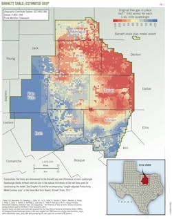
Original gas in place (OGIP) is mapped with 1-square-mile grid blocks. Total free OGIP for the 8,000-square-mile study area is 444 tcf, with about 280 tcf in blocks drilled by the end of 2010 (Fig. 1).

We then used the EUR calculated for every well, combined with reservoir volumetrics, to quantify the volume of reservoir drained by each well.2 We call the surface expression of this volume "drainage area" and represent it by a rectangle on a map.
We recognize that actual drainage areas are not ideal rectangles and that the combination of hydraulic and natural fractures can extend production reach farther than one location away, but rectangles provide an acceptable shape that is somewhat consistent with microseismic results, as well as a means of accounting for the drained volume.
At this stage, it was unclear whether wells drained a large volume with a small RF or a small volume with a large RF to achieve the estimated EUR calculated for a given well.
To determine RF, we developed a mathematical procedure relying on production data.
First, we varied the RF for every well, allowing the resulting drainage area to expand and contract. Then, for every instance in which closely spaced wells began to have overlapping theoretical drainage areas, we checked whether the initial well's actual production decline experienced interference when the second well began producing.
We then varied the RF and resulting drainage area until the theoretically predicted overlap in drainage areas best explained the observed production interference between closely spaced wells. If the assumed RF was too low, large areas of overlapping drainage would be indicated, when wells clearly did not actually interfere. If the assumed RF was too high, no overlap would be indicated between wells that did interfere.
By applying this approach to all vertical wells and, separately, to all horizontal wells, we determined that a 45% RF best explained vertical-well interference and a 55% RF best explained horizontal-well interference. These individual recovery factors are somewhat higher than we expected.
Implicit in RF analysis is an assumption about the shape and orientation of the drainage area. A plot of horizontal-well EUR vs. well orientation for all wells clearly shows a minimum at NE 55° azimuth, indicating the prevailing principal horizontal stress direction in which fractures most readily propagate. Accordingly, we oriented vertical-well drainage areas at this angle.
We also were able to find empirically that the length:width ratio for the drainage areas of vertical wells is close to 1.5:1, an estimate consistent with those of microseismic examples in the field. For horizontal wells, we assumed a drainage area as long as the horizontal section in the reservoir and having a width consistent with the EUR and RF, as discussed earlier.
The RFs obtained, however, cannot be readily applied to the entire field. The distribution of wells is not even—better tiers are much more densely drilled than are lower tiers so that about 85% of all interfering wells are from Tiers 1-4.
To find RFs for lower quality productivity tiers, we used permeability derived for each tier.2 Thus, for Tiers 5-10, we assumed that RF decreases roughly in proportion to permeability such that in Tier 10, RF will decrease by about 10x.
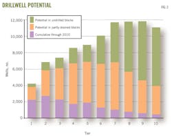
From drainage-area calculations for every well, we were able to approximate the amount of drained and undrained acreage for each square mile of reservoir. Then, knowing the undrained acreage remaining in each square mile, we created an inventory of future feasible drilling locations (Fig. 2). The better tiers are more developed, and the lower tiers, except where liquids production is high, remain uneconomic at almost any foreseeable gas price.
Well economics
We analyzed the production history of every well in each tier and determined average well profiles in each rock quality tier.2 The EURs of every well were determined with linear transient-flow-decline equations and including the dampening effect of interfracture interference assumed beyond Year 8. An average production profile for a 4,000-ft horizontal well was developed for each tier based on historical data from wells in that tier.
These production profiles formed the foundation for future production modeling in each tier (Fig. 3). We further modified these profiles in the production model to account for attrition effects, pace of technology improvement, and deterioration in well quality due to crowding as development entered its later stages.

The study looks at average EUR per well per tier, assuming a 25-year well life (Table 1). For the top five tiers, which are most important for the field, about 50% of EUR is recovered during the first 5 years, roughly 73% in first 10 years, and 86% in first 15 years. The actual average EUR recovered will be lower because attrition and economic limits will prevent some wells from producing for the full 25 years (Table 2).
The study's production model includes the effect of historical attrition rates (separately for wet and dry-gas areas), which were found to increase as the rock-quality tier decreased. These findings indicate the importance of understanding the distribution of rock quality for economics of future drilling and production forecasts and the risks of using a single field-wide average.

The average well profile in each tier is used to estimate average well economics. We developed a representative group of well economic parameters that was reality-checked and mostly validated with detailed input from several operators in Barnett field (Tables 3 and 4). The economics are sensitive to the btu content of natural gas production, so that ultimately the study subdivided the field into a high-btu (>1,100 btu) area to the west and a low-btu (<1,100 btu) area to the east, as mapped by Bruner and Smosna.3

We developed a comprehensive well-cash-flow model to determine the internal rate of return (IRR %) for an average well in each tier of both the dry-gas and wet-gas areas of the field (Fig. 4).
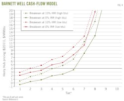
The high liquids content improves well economics significantly, in comparison with production of dry gas, for an equivalent-quality tier. In recent years, lower natural gas prices and rising oil prices have caused drilling activity to shift to the western part of the field. A full range of price sensitivities, to determine how IRR % is affected by changes in input assumptions, is described elsewhere.4
Production outlook
On the basis of the productivity tier map, inventory of future well locations available in each tier, and an understanding of the economics of an average new well in each tier, we next modeled the pace of future development activity in the field.5 An "activity-based model" allows for new drilling based on available-location inventory. The model adjusts the pace of activity annually, constrained by the economics of the average well in a given tier.
On the basis of the differing economic incentives, the model is subdivided according to tier and whether the well is in a dry or wet-gas area. The historical pace of drilling as it changed across the range of historical prices helps scale the model's reaction to changing price. The model tracks the number of wells drilled in each tier each year and totals the production effect using average well profiles by tier, which incorporate decline profiles (assuming linear flow in the reservoir).
The production effect of new drilling activity is then layered on top of the extrapolated production decline of all historical wells drilled. In other words, the model accounts for the observed inertia of drilling to predict how the pace of drilling will increase or decrease as a function of price incentive (change in IRR%) and size of the remaining well inventory.
The model has the ability to vary many parameters besides well price. It can, for instance, withhold acreage from development that is due to surface limitations or spacing inefficiencies such as leasing obstacles. The result is a forecast of future completions from the field through 2030 and a resulting full-field EUR through 2050 for any set of assumed parameters.
The model is driven by assumptions that include:
• Average well declines specific for each tier.
• Effects of late-life deterioration in decline.
• Effects of attrition.
• Maximum 25-year life assumed for all wells.
Also in the base-case scenario, we allow development of a maximum of 80% of the acreage in currently producing blocks but only 15% of the acreage in undeveloped blocks. We also set minimum activity levels in each tier, reflecting past performance in low-price periods, and incorporate several other assumptions (Table 5).

Given the base set of assumptions, the model generates a production forecast (Fig. 5). In the environment of a $4/MMbtu natural gas price at Henry Hub (HH), production reaches a plateau between 2012 and 2015 and begins a gradual decline as annual well count decreases as a function of limited higher-quality drilling locations.
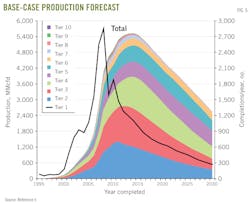
These locations in Tiers 1-4 are developed, and the lower tiers, with the exception of areas of higher btu content, do not justify development at this price. The outlook yields a full-field EUR of 45 tcf, which includes the 18.5 tcf expected from 15,144 wells drilled through 2010.
The production outlook and resulting EUR are only moderately sensitive to natural gas price (Fig. 6). Higher prices will extend the buildup and plateau period.
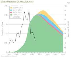
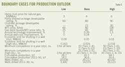
Natural gas price is only one of several variables. We developed low and high cases around the base to capture the impact of other key variables (Table 6).
We also developed a stochastic simulation analysis to vary an array of input variables over reasonable distribution ranges, accounting for correlations between variables. This stochastic approach provides a sense of the range of EUR outcomes and accompanying risk that can be expected from Barnett field (Fig. 7).
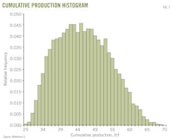
The mean of the resulting distribution is 46.5 tcf, which is slightly higher than our base case estimate primarily because the historical natural gas price distribution we use for simulation has a mean of $5.36/MMbtu. It is worth noting that our worst-case scenario is unlikely to occur. Similarly, our high case scenario has about 1% probability of occurring.
Implications
The multi-disciplinary, bottom-up approach summarized in this two-part series represents a new approach to current public practices for reserve and production forecasting in unconventional shale-gas reservoirs. Our team has nearly completed similar studies in the Fayetteville, Haynesville, and Marcellus, and will deploy a similar approach in two major shale oil basins beginning in 2014.
Although it would be difficult to approach all basins with this level of detail, the results provide a benchmark with which to compare more general, top-down approaches. Results of this work have implications for discussions regarding balance of trade, regulation and infrastructure planning, carbon and methane emissions, and energy security.
References
1. "Review of Emerging Resources: U.S. Shale gas and Shale Oil Plays," US Energy Information Administration, Department of Energy, July 2011.
2. Ikonnikova, S., Browning, J., Horvath, S., and Tinker, S.W., "Well Recovery, Drainage Area, and Future Drill-well Inventory: Empirical Study of the Barnett shale Gas Play," SPE Reservoir Evaluation & Engineering, under review.
3. Gülen, G., Browning, J., Ikonnikova, S. and Tinker, S.W., "Barnett well economics," Energy, forthcoming.
4. Bruner, K.R., and Smosna, R., "A comparative study of the Mississippian Barnett shale, Fort Worth Basin, and Devonian Marcellus shale, Appalachian Basin," US Department of Energy, National Energy Technology Laboratory, DOE/NETL-2011/1478.
5. Browning, J., Ikonnikova, S., Gülen, G., and Tinker, S.W., "Barnett shale Production Outlook," SPE Economics and Management, July 10, 2013.