NORTH AMERICAN RESOURCE VALUE—1: Economics, fiscal competitiveness eyed for Canada, US tight oil plays

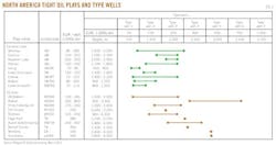
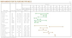
Fig. 1 identifies the type well estimated ultimate recoveries (EURs) selected for Part I. While the type wells for the individual play analysis in Part II are consistent with those of Part I, the Part II type wells will reflect more closely the specific parameters and expectations for the individual plays.

The North American type wells for Part I are designed to be representative by reflecting the range of EURs reported publically for each individual play identified. Two important observations are highlighted at this point: (a) the EURs for the US plays tend to be higher than those for the Canadian plays, and (b) the depths of the Canadian plays tend to be shallower than those for the US plays.

What is tight oil?

The Canadian Society for Unconventional Resources (CSUR) defines tight oil as "conventional oil found within reservoirs with low permeability.

"The oil contained within these reservoirs typically will not flow to the wellbore at economic rates without assistance from technologically advanced drilling and completion processes. Commonly, horizontal drilling coupled with multistage fracturing is used to access these difficult to produce resources."

The terms "tight oil" and "shale oil" are used interchangeably, however tight oil is sometimes referred to as tight-light oil to distinguish it from oil shale. Oil shale is not the same as shale oil—there is a huge difference. The following definition from Gue 2010 is helpful in making the distinction.

"Liquid crude oil consists of organic material—plant and animal remains—that's been exposed to heat and pressure over millions of years. The slow transformation of organic material into oil progresses through a number of stages. Kerogen is a solid organic compound that occurs relatively early in this process. To understand where kerogen fits into the developmental timeline, consider that bitumen—the hydrocarbon found in Canada's oil sands—represents a later stage in the process. In a sense, bitumen is a higher-quality and more useful hydrocarbon than kerogen. Oil shale is an inorganic rock that contains kerogen. The term oil shale is a misnomer because kerogen isn't crude oil, and the rock holding the kerogen often isn't even shale. To generate liquid oil synthetically from oil shale, the kerogen-rich rock is heated to as high as 950° F. (500° C.) in the absence of oxygen, a process known as retorting."¹

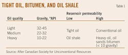
Table 1 and Fig. 2 provide further illustration, first in the context of the conventional oil classification light-heavy-extra heavy-bitumen (Table 1) and then in terms of different permeabilities associated with different types of source rock (Fig. 2).

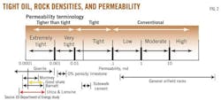
The tight oil source rock has a permeability that is lower than sidewalk cement and comparable to granite. This is why the fracturing technology is essential to creating conditions where the oil can flow to the wellbore.

Crude oil price assumptions

The base case crude oil price is modeled at (US) $85/bbl for West Texas Intermediate (WTI).

Due to the generally low tight oil densities, no adjustment is made for quality. Transportation costs are modeled at $5/bbl, for a netback price to the field of $80/bbl.

Limited price sensitivity is performed in Part I, however Part II incorporates extensive price sensitivity analysis in order to provide estimates of the break even supply prices for each play.

Type wells

Tight oil type well production profiles

Actual production profiles for a given play typically exhibit significant and extreme variability from period to period and across different wells, and this variability can be even more pronounced for resource plays that involve multiple stage hydraulic fracturing.

While the production profiles for the type wells reflect a smooth decline that is uncharacteristic of actual experience, they are nevertheless useful in establishing context and removing some of the daily production rate "noise" that would otherwise make it more difficult to identify the more general and longer term economic effects.

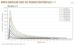
The effects of real production profile and EUR variability are accommodated through the choice of a wide EUR range for the type wells and by sensitivity analysis for each well.

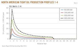
Following a hyperbolic decline distribution characteristic of tight oil and gas, the annual production profiles associated with each of the seven type wells are presented in Figs. 3 and 4. Fig. 4 is simply a subset of Fig. 3 to better illustrate the nature of the profiles for the lower EUR wells.

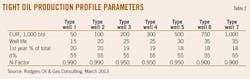
Table 2 presents the well life and annual decline parameters used to generate each type well production profile.

Well costs

Cost in this section means "technical costs"—the unrisked capital and operating expenditures, excluding the cost of unsuccessful wells, dry holes, payments to governments, and the return required by investors.

These costs are incorporated through the economic analysis—bonus payments for land in the payments to government, rate of return through the discount rate, and dry holes through expected monetary value (EMV) analysis. EMV analysis is not incorporated into this report.

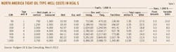
Included in the capital costs (CapEx) are geological and geophysical expenses, the successful well drilling, completion, and tie-in, production facilities, and the cost of abandonment and reclamation. Operating costs (OpEx) include fixed and variable components, well work-over costs, water handling costs, a cost allocation for general and administrative expenses, and an allocation for costs to a major transportation point. Where required, CapEx and OpEx would also include costs related to the handling of solution gas. Table 3 presents the CapEx and OpEx for each type well.

Fiscal systems

Each tight oil type well is assessed under 19 fiscal systems representing the 13 jurisdictions selected. They are, in Canada, British Columbia (2), Alberta (1), Saskatchewan (1), Manitoba (1), and Newfoundland (1), and in the US, California (2), Colorado (2), Louisiana (1), New Mexico (2), Montana (2), North Dakota (1), Wyoming (2), and Texas (1). For British Columbia, two fiscal systems are assessed, the light oil Third Tier vintage system and the net profits royalty (NPR) system.

Finally, the fiscal system applicable in onshore Newfoundland is included as prospective tight oil resources have been identified on the province's west coast.

For the US jurisdictions, distinction is made between federal lands and private lands.

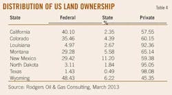
The US systems included for each state are selected on the basis of the significance of land ownership between federal, state, and private lands (Table 4). On this basis, and because there are generally no significant differences between the fiscal terms for state lands and those for private lands, only federal and private lands are included.

Including federal lands is useful not only because there is a significant portion of federal land ownership in many states but also because the lower royalties on these lands provide a sense of the economics for wildcat exploration areas and for emerging plays that have not yet matured to become generally attractive development properties. In these situations private and state lease terms can see lower royalties, however typically not as low as those on federal lands.

Explanations for the lower royalty rate on federal lands include the US's position as a net importer of oil and gas and the consequent policy to encourage domestic production.

Type well economics

Table 5 shows for each type well the unburdened (no government) results for the selected economics decision-making criteria.

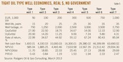
All wells are shown to have attractive economics with rates of return ranging from 22.99% to 85.04% and discounted ratios of profit to investment, or PIR10s, ranging from 0.43 to 2.47.

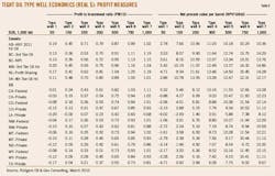
Tables 6 and 7 present selected economics and fiscal indicators under the fiscal terms applicable to each jurisdiction.

Reviewing the results in Table 6 reveals that a new well in the US with an EUR of 50,000 bbl under the modeled cost and price assumptions would be subeconomic with a PIR10 less than zero except for California federal lands where the well is shown to be marginally economic. This observation extends to the 100,000-bbl case for Louisiana. The NPV10 per barrel results support this conclusion.

It is noted that the costs modeled are full cycle. Thus, they represent an entry well in a new play. Half-cycle costs, which would be more representative of an entire play, would be lower and therefore yield improved economics.

For a given EUR size, the Canadian systems all record improved economic attractiveness when compared to the US systems. This results from the generally lower government share in Canada and the front-end loaded nature of the US systems.

Government share, often referred to as government take, refers to the percentage of net revenue (revenue less CapEx and OpEx) that is captured by government. Government includes all levels: federal, state-provincial, and county-municipal. It also includes the share paid to private landowners.

Components of the government share include bonus payments, royalties, corporate income tax, and property tax.

The government shares are compared in Table 7, which shows the share in percentage terms and in terms of cost per barrel. Government share is discussed further below.

It is highlighted that the level of government take is not a reliable criterion for determining the economic attractiveness of a given investment prospect or the competitiveness of a particular jurisdiction. This is especially true for fiscal systems that are highly dependent on fixed up-front royalties and severance taxes.

When judging economic attractiveness and competitiveness, government share should be considered only in association with more appropriate investment criteria such as rate of return, profit to investment ratio (PIR), and net present value (NPV).

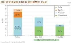
The limitation of government share as an economic decision-making criterion is illustrated in Fig. 5 below. Fig. 5 shows, first for the "no government" case, the distribution of project price among OpEx, CapEx, and per tax net revenue (the net revenue available for sharing). The figure then shows the distribution of net revenue between the producer (49%) and government (51%). Finally, with all other variables held constant, the change in these shares as a result of an increase in costs is shown.

For this illustrative example, and assuming no offsetting fiscal effects, a cost increase from $26/bbl to $50/bbl increases the government share to 84%. This shows that under ad valorem royalty systems the government share can increase even though tax and royalty rates are held constant.

The government take may indeed be high because of high tax and royalty rates, however even low ad valorem royalty rates and other nonprofit-sensitive fiscal elements can produce a high government share if costs are high or revenue is low. It is precisely because of these cost effects that many jurisdictions employ profit-based systems such as those based on rate of return; e.g., BCs, NPR, and NL.

Fiscal systems competitiveness

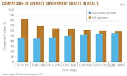
Fig. 6 compares the average government share for Canadian and US jurisdictions:

• US systems are consistently regressive, while Canadian systems are progressive, taking a higher percentage share as profitability increases.

• While progressive systems match better with economic principles including that of not altering the investment decision, regressive systems trade off the encouragement of cost control and innovation with otherwise lower levels of industry activity.

• The US systems generally take a higher share than the Canadian systems—the fiscal costs in Canada are lower than in the US. Selecting the medium EUR case for illustration, the average US government share is 61.1% compared with 44.8% for Canada.

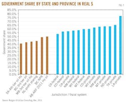
Looking at the government share by state and province is also revealing. Fig. 7 compares the shares by fiscal system for the medium EUR case:

• The highest share is clearly recorded for Louisiana (76.95%). The high share for Louisiana is attributed to relatively high rates for severance tax and property tax.

• The share for Texas is 65.08%.

• There is a clear separation of the Canadian and US systems.

• The highest Canadian share is lower than the lowest US share.

• Alberta has the highest share of the Canadian jurisdictions (50.03%). The British Columbia NPR terms are included only for reference, as these terms are so far not being applied to tight oil and are limited only to Horn River shale gas.

• Saskatchewan represents the lowest overall Canadian share at 40.71%.

• The lowest US share is on federal lands in California (53.15%).

Fiscal system component analysis

This section is an analysis of the impact of the various components of each fiscal system.

It is noted that the US systems all have the same basic structure, with some modifications around the base for the property tax. Some states have property tax based on the value of the remaining resource; e.g., Texas, while others base their property tax on the value of the facilities and equipment; e.g., Montana and Louisiana.

Because of the similarities across states only the systems for Texas and Montana are assessed on a subcomponent basis. All of the identified Canadian systems are assessed because they all exhibit quite different fiscal structures.

For the Canadian systems, property tax is not modeled as a specific fiscal component. It is instead included in the operating costs. Property tax in Canada is relatively insignificant when compared to the other fiscal instruments such as royalties, and it is well within the tolerances of the cost assumptions for this analysis.

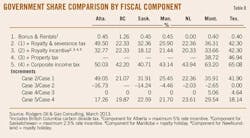
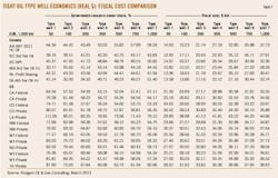
Table 8 summarizes the incremental component results for the selected fiscal systems. The following observations are highlighted:

• The share of government take attributable to bonuses and rentals is comparable. Bonus payments in this analysis are held constant across all jurisdictions. This is to facilitate comparison of the fiscal elements that are controlled by governments. Investors have full control of the amount they bid. One would expect that projects with higher profitability would attract higher bids. British Columbia's share includes the CO2 tax, and Newfoundland requires neither bonuses nor rentals.

• Alberta's base royalty share is clearly higher than that of the other jurisdictions. Incentives however lower the share by almost 17 percentage points, bringing the overall share before corporate income tax (CIT) from 49.50% to 32.77%. The royalty share in Alberta is based on an elaborate equation involving price, productive zone, production rate, holiday-volume and holiday-time. The holiday is based on the total measured depth (TMD) of the well. The TMD is in turn dependent on the TVD and on the length and number of lateral well segments.

• After incentives, Alberta's royalty share is about 10 percentage points lower than that of Texas but still higher than that for the other Canadian jurisdictions.

• When US style property tax is added the before tax share in Texas is about 14 percentage points higher than the highest Canadian share (AB) and 29 percentage points higher than the lowest Canadian share (SK).

• When corporate income tax is added, the overall government share in Texas increases to 65.1% compared to 50.0% in Alberta. While the CIT rate is significantly higher in the US—35.62% for Texas compared with 25% for Alberta—the difference in overall government share increases only marginally from 14 to 15 percentage points. This is related to the higher deductions available under the US system as a result of higher royalties, severance tax, and property tax.

The higher overall fiscal cost in Texas, for example and generally in the US, is interesting. This is often attributed to generally lower costs in the US, thus making higher government shares economically possible. While this is no doubt part of the explanation, it does not appear to be the full story.

Other aspects of the explanation relate to a generally high rate charged by private land owners versus governments. Unlike private landowners, governments are often concerned with maintaining or even increasing the level of industry activity and employment, thus opting for a somewhat lower share of direct revenues.

Another aspect of the explanation is that higher tax rates mean that the US jurisdictions effectively bear a higher share of risk investments, such as the costs for land acquisition, seismic acquisition, exploration dry holes, and research. Of course this front-end effect is balanced by a higher tax burden on project profits.

Yet another part of the explanation relates to the high front-end nature of the US systems, particularly on private lands. The "hard bargain" driven by private landowners and relatively high upfront fixed royalties represents added incentive for US producers to innovate and lower costs.

To acquire some additional context for considering the fiscal cost of doing business it is helpful to compare the various fiscal systems on a cost per barrel basis. This facilitates direct comparison with a more commonly understood metric such as the CapEx cost per barrel or the per barrel price.

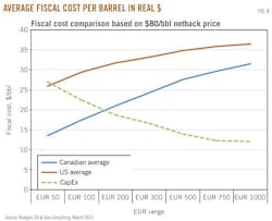
Fig. 8 shows the US and Canadian government shares expressed in US dollars per bbl. The average fiscal cost is clearly lower in Canada, by $5 to $13/bbl for the EUR 1000 and EUR 50 cases, respectively. This is a sizable difference when compared to CapEx for this case at $16.67/bbl. The additional government share per well in the US represents a value comparable to 30% to 78% of the overall CapEx.

Further sense of the Canadian fiscal advantage can be obtained from the data in Table 7. It can be seen from the results for Type well 4 that, for example, the fiscal cost in Alberta is $27/bbl compared with $34/bbl in Montana, and $22/bbl in Saskatchewan compared with $34/bbl in North Dakota. The fiscal advantage in Alberta is enough to pay for over 40% of base case well costs. This share increases to over 70% in the case of Saskatchewan.

Fig. 8 also shows that the difference between the US and Canadian systems narrows as profitability increases. This is due to the progressive nature of the Canadian systems with rates based on profitability or a proxy for profitability through changing production volumes and price. Alberta is a good example, where the royalty rate is a function of both price and quantity.

Table 7 shows that over the range of EURs, Alberta's share increases from 44% to 59%. The corresponding share for Texas decreases from 88% to 61%. The difference between the two systems shrinks from 44% in the EUR 50 case to only 2% in the EUR 1000 case.

A similar effect occurs with changing prices. Table 9 compares Alberta, British Columbia, and Texas for changes in price from (US) $60/bbl to (US) $100/bbl.

While the results from Table 7 showed AB's system to be clearly progressive with respect to production, Table 9 shows the overall system to be essentially neutral over the selected range with respect to changes in price. British Columbia's system showed slight progressivity across the EUR range but is modestly regressive over the modeled price range. For Texas, changes in price show a comparable level of regressivity as that exhibited across the EUR range.

Next: PART II will be a discussion of the economics of individual tight oil plays. It will also add further perspective on the issue of fiscal costs, placing these costs in the broader context of the overall costs and economic attractiveness of each play.

Reference

1. Gue, Elliott, "Oil Shale, Shale Oil, and 6 Ways to Play the Difference," Seeking Alpha, November 2010.

The author

Barry Rodgers ([email protected]) is president of Rodgers Oil & Gas Consulting in Edmonton, Alberta, Canada. He has more than 30 years of energy industry experience, specializing in upstream economics and fiscal system design. He has advised private sector investors and host governments and has served in a number of international advisory roles. Most recently Rodgers Oil & Gas Consulting has coproduced World Fiscal Systems for Oil & Gas covering 156 countries. Rodgers is a graduate of Memorial University.