Regression models estimate pipeline construction costs
Zhenhua Rui
Paul A. Metz
Douglas B. Reynolds
Gang Chen
Xiyu Zhou
University of Alaska-Fairbanks
Fairbanks, Alas.
This article develops five regression models to estimate pipeline construction component costs for different types of pipelines in different regions. It then uses the regression results to investigate cost differences between regions, pipeline cross-sectional area, and pipeline length.
Background
Researchers have long used historical pipeline cost data to estimate the projected construction costs of different types of future pipelines.1-5 Such data allowed development of five pipeline construction-component cost estimation models in this article with multiple nonlinear regression, with various statistical tests confirming the models as valid. The models estimate pipeline construction component costs with respect to different pipeline cross-sectional areas, lengths, and regions, with results showing a large cost difference between regions.
Analysis found the economy of concentration to be an important factor in reducing cost, while the Cobb-Douglas function assesses the relationship between pipeline cost and pipeline cross-sectional area and length, showing economies of scale in most pipeline costs components. Cost estimation models, however, encounter limitations due to missing information such as pipeline WT.
Data set
Data availability guided pipeline selection, with pipeline cost data collected from Oil & Gas Journal's annual data book. Limited offshore pipeline data led to the collection of data for onshore pipelines only. Pipeline costs in this article do not include compressor station costs.
The pipeline data set includes the year of completion, pipeline OD, pipeline lengths, pipeline locations, and pipeline construction component cost. Pipelines from all 48 of the contiguous US states appear in the data set, with Alaska and Hawaii excluded. The data set also contains 15 Canadian pipelines. Completion of the pipelines took place between 1992 and 2008. Cost is real, accounted costs determined at the time of completion.
The entire data set consists of 412 onshore pipelines. The five pipeline construction cost components are: material, labor, miscellaneous, right-of-way (ROW), and total cost.
Material cost is the cost of line pipe, pipeline coating and cathodic protection. Labor cost consists of the cost of pipeline construction labor. Miscellaneous cost is a composite of the costs of surveying, engineering, supervision, contingencies, telecommunications equipment, freight, taxes, allowances for funds used during construction, administration and overheads, and regulatory filing fees. ROW cost contains the cost of ROW and allowance for damages.
Total cost is the sum of material cost, labor cost, miscellaneous cost and ROW cost.5 Cost adjustments used the Chemical Engineering Plant Cost Index—a widely used index for adjusting process plants' construction cost—to 2008 dollars.6
Location information for US pipelines in the data is by state. The US Energy Information Administration (EIA) breaks down the US natural gas pipeline network into six regions: Northeast, Southeast, Midwest, Southwest, Central, and Western (Fig. 1). State grouping is based on 10 federal regions of the US Bureau of Labor Statistics.7 These regional definitions are used to analyze geographic cost differences,4 with the 15 Canadian pipelines assigned a separate Canada region.
Developing models
The data set's inclusion of information on pipeline length, OD, and location prompted use of the multiple nonlinear regression method. Using pipeline cross-sectional area as a variable instead of pipeline diameters allowed more accurate evaluation of the relationship between pipeline construction component costs and the pipeline's physical parameters. Cost components adjustment to 2008 dollars used different categorical chemical indexes instead of just the composite index.
Equation 1 shows the general form of the multiple nonlinear regression used to build the individual categorical costs.
The positive of αi of regional variables shows a region has a lower cost than the Central region.
Equation 1 provided the basis for developing five cost estimation models. Table 1 shows coefficients of the regression models.
Validating models
Some tests occurred before building the regression model. Table 2 shows the results of these tests.
Examining the independent variables in the model for mulitcollinearity comprised part of the testing. The variance inflation factor (VIF) is a diagnostic applied to test the independent variables. The VIF values of independent variables in these five models are between 1 and 1.7 (Table 2). A VIF value under 10 is generally acceptable.8 The independent variables therefore do not have a mulitcollinearity problem.
An F test and its associated p-value test the overall model for predictive capability. The ratio of the mean of the square for regression and the mean square for error is called F-statistics.9 Normally a large F-value suggests that the model explains a large proportion of variance. The p-value associated with the F-statistic is considered very significant when the p-value is less than 5%. F-statistics of all five models are very large, and associated p-values are less than 1% (Table 2), leading to the conclusion that at least one of the parameters in the model has a predictive capability. All p-values of coefficients are below 5% (Table 1), allowing consideration of all parameters in these five models as significant.
R-square and adjusted R-square are diagnostics that help determine the model's goodness-of-fit. The R-square shows the proportion of variance in the dependent variables as explained by the independent variables. One disadvantage of R-square is its value can be artificially inflated by putting in additional independent variables.10
Adjusted R-square, therefore, is often used with R-square. The values of R-square of all models are greater than 0.75, and the adjusted square values are almost the same as that of the R-square in all models (Table 2), showing a large proportion of variability as explainable by the independent variables and the regression models' validity.
Assumption of normality claims residuals need to fit the normal distribution. The Shapiro-Wilk (SW) test is a quantitative test to evaluate the normal distribution's goodness of fit.8 The null hypothesis of the SW test is a normal data distribution.
The p-values produced by SW tests of labor, miscellaneous, and total cost data are greater than 5% (Table 2), consistent with the null hypothesis. Material and ROW data are 3.6% and 4.1%, respectively, slightly less than the 5% threshold. But the magnitude of these violations is deemed reasonable. Assumptions of normality for all models, therefore, are reasonably satisfied.
Another assumption for the regressions is the homoscedasticity of residuals. The Breusch-Pagan (BP) test is a quantitative test for homoscedasticity.8 The null hypothesis of the BP test has the residual in constant variance. The BP test also produces a p-value. All p-values of BP tests in the five models are greater than 5% (Table 2), the null hypothesis is not rejected, and the constant variance is satisfied.
The diagnostics, therefore, demonstrate the validity of the five regression models. The following sections will use regression models to analyze cost difference in terms of regions, pipeline cross-sectional area, and pipeline length.
Regional differences
Regional coefficients show the cost differences in different regions (Table 1). Coefficients of these regions show all location-related pipeline construction component costs.
The material cost model shows a relationship to the Southeast, Midwest, and Canada regions. Material costs in the Midwest and Canada are lower than the Central region, according to the sign of coefficients, while material costs in the Southeast are much higher than in the Central.
The labor cost model shows a relationship to all regions except Canada, and the labor costs in other regions are higher than in the Central region. The Northeast has the highest labor cost.
The miscellaneous cost model displays a relationship to the Northeast, Southeast, Midwest, and Southwest, and all coefficients are positive. The Southeast has the highest miscellaneous cost.
ROW cost and total cost models show relationships to all regions, and all coefficients are positive except for Canada. The Midwest and Southwest regions have the first and second highest ROW cost. The Southeast has the highest total cost. Canada has the lowest total cost and the lowest ROW cost.
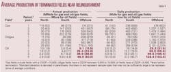
For comparison purposes, using cost estimation models, Table 3 gives unit total cost of 24 in. OD pipe for 100-mile pipeline construction segments in different regions. Unit total cost of the pipeline in different locations varies noticeably. The unit total cost in Canada, for example, is $29.60/cu ft, but unit total cost in the Southeast is $76.60/cu ft. Southeast region pipeline unit total costs are 2.6 times the pipeline unit total cost in Canada and 1.8 times the pipeline unit total cost in the Central. The cost difference for pipeline construction caused by geography can sometimes reach 300%. The geographic factor, therefore, is important in determining pipeline cost.
Seen from the values of the coefficient of Southeast and Northeast regions, the Northeast has a higher cost of living than the Southeast. The Southeast actually has higher miscellaneous, ROW, and total costs than the Northeast but slightly lower labor cost.
This comparison may show an economy of concentration playing an important role in pipeline construction cost. An economy of concentration is one type of economy of scale, also called external economies. Economy of scale tends to arise when firms or projects in the same industry are close together.11 Roughly 40% of US pipelines are in the Northeast, and 46% of them are concentrated in Pennsylvania. These concentrations reduce pipeline construction cost.
Cost differences between regions are caused by two main types of factors:4
• Differences in material and ROW cost.
• Geographic factors, such as terrain and population density.
Weather conditions, soil properties, cost of living, and distance from supplies are also regional variables which can cause cost differences.12 Conducting quantitative analysis of cost difference in different locations, however, is impossible without pipeline-related information such as pipeline route.
Pipe differences
Coefficient results show cost is also related to pipeline cross-sectional area and pipeline length. The Cobb-Douglas function serves widely as a production function representing the relationship between input and output. The Cobb-Douglas function has interpreted cost in terms of pipeline size and length.4 In this article the function will explain the relationship between cost and pipeline cross-sectional area and length.
Equation 1 can be written in Cobb-Douglas form as Equation 2.
The partial derivative ∂c/∂s is the rate at which cost changes with respect to pipeline cross-sectional area: marginal cost with respect to pipeline cross-sectional area. Likewise, the partial derivative ∂C/∂L is the rate at which cost changes with respect to pipeline length, and is called marginal cost with respect to pipeline length. The marginal cost with respect to pipeline cross-sectional area is proportional to the amount of cost per unit of pipeline cross-sectional area. The marginal cost with respect to pipeline length is proportional to the amount of cost per unit of pipeline length.
The Cobb-Douglas function is well known for its return to scale (Equation 3).11 If the sum of α7 and α8 is 1, the cost function has constant returns to scale. If the sum of α7 and α8 is less than 1, the cost function has decreasing return to scale, and if the sum of α7 and α8 is larger than 1, the cost function has increasing return to scale.11
Table 2 shows that sums of α7 and α8 in the five models are all greater than 1, so all five component cost models have increasing return to scale. That is, if both cross-sectional area and length are increased by m times, the cost will increase more than m times.
But both α7 and α8 are smaller than 1 for material cost, labor cost, miscellaneous cost, and total cost. These cost models have increasing returns to scale with diminishing marginal cost, which means that the rate of pipeline cost increase is less rapid than the rate of the pipeline area or rate of the pipeline length increase.
The ROW cost model is a nonsymmetric function with increasing returns to scale, because α7 is smaller than 1 and α8 is bigger than 1, the rate of pipeline cost increase is less rapid than the rate of pipeline cross-sectional area increase, but the rate of pipeline cost is more rapid than the rate of the pipeline length increase. For example, when pipeline length doubles, the material cost is less than double, while the ROW cost increase more than doubles.

All cost components therefore have economy of scale with respect to pipeline cross-sectional area, and all cost components have economy of scale with respect to pipeline length except for ROW cost. The coefficient of pipeline length in the ROW cost model is almost 1. ROW cost almost doubles when pipeline length doubles, showing a near-constant ROW unit regardless of length.4

Figs. 2-6 show estimated pipeline unit component costs in the Central region, demonstrating the trend of pipeline component cost regarding pipeline cross-sectional area and pipeline length. Fig. 2 shows pipeline unit total cost decreasing as pipeline length and pipeline cross-sectional area increase, supporting the conclusion that total cost has economy of scale with respect to pipeline cross-sectional area and length. For example, the unit total cost of 8-in. OD pipelines is 6.2 times 48-in. pipelines, and the unit total cost of 50-mile pipelines is 1.7 times 800-miles pipelines. A similar trend exists in material, labor, and miscellaneous cost (Fig. 3, Fig. 4, and Fig. 5, respectively).
Fig. 6 shows the trend of estimated pipeline unit ROW cost in the Central region. The pipeline unit ROW cost decreases as pipeline cross-sectional area increases, while the pipeline unit ROW cost slightly increases as pipeline length increases. This shows ROW cost as having economy of scale for pipeline cross-sectional area, but not for pipeline length. All component costs, therefore, have economy of scale regarding both pipeline cross-sectional area and length, except ROW, which only has economy of scale with respect to cross-sectional area.
The economy of scale caused by growth of a project is called internal economy of scale. For pipeline projects, internal economy of scale is created by increasing pipeline cross-sectional area and pipeline length.
The four main categories of internal economy of scale are: technical economies, managerial economies, marketing economies, and financial economies.11 Technical economies use specialized equipment or processes to improve labor and capital productivity in large pipeline projects. For example, large and efficient trenchers are employed to increase productivity and reduce the cost of diesel and carbide teeth. Many small pipeline projects cannot afford an initial heavy investment due to the inability to diffuse high fixed costs.
Managerial economies manifest themselves when large pipeline projects hire professional and specialized mangers for separate tasks instead of relying on one general manger to take care of everything. Marketing economies manifest themselves in discounts realized by buying materials in huge quantities, while lower interest rates or greater government assistance stand as examples of financial economies likely to be granted to large pipeline projects.
These explanations support the idea that large pipeline projects have economy of scale and low unit cost. The explanations also match the regression results that unit costs of pipeline construction components fall with increasing pipeline cross-sectional area and length, except for ROW cost, which only decreases with increasing cross-sectional area.
Analysis limitation
The data used in this article include a large number of pipelines built between 1992 and 2008, but there are still not enough pipelines in some regions, such as Canada and the Western region, to form a representative sample. Pipelines in these regions show less correlation to pipeline construction component costs compared with other regions.
In the data set, 78% of pipelines are less than 60 miles long.13 The relative lack of long pipelines may cause estimation biases. Cost data also do not provide the year construction started or the construction period, which causes cost biases when adjusting with the chemical plant index.
US natural gas pipelines' region definitions are based on federal regions of the US Bureau of Labor Statistics. Region definitions of natural gas pipeline systems could instead be made according to geographic similarity, cost of living, or other criteria. Some important variables also remain missing, such as pipeline WT, steel grade, maximum allowable operating pressure, terrain along the pipeline route, and ownership type, any of which could produce cost differences.
Future work should collect more observations in Canada and Western regions and for long pipelines, more information about project construction schedules, and more data on the missing variables.
References
1. Parker, N., "Using natural gas transmission pipeline costs to estimate hydrogen pipeline costs," UCD-ITS-RR-04-35, 2004.
2. Zhao, J., "Diffusion, costs and learning in the development of international gas transmission lines," International Institute for Applied Systems Analysis, IR-00-054, 2000.
3. Heddle, G., Herzog, H., and Klett, M., "The economics of CO2Storage," MIT LFE, 2003.
4. McCoy, S.T., and Rubin, E.S., "An engineering-economic model of pipeline transport of CO2with application to carbon capture and storage," International Journal of Greenhouse Gas Control, Vol. 2, No. 2, pp. 219-229, 2008.
5. Oil & Gas Journal Databook, Tulsa: PennWell Corp., 1992-2010.
6. Chemical Engineering, Plant cost index, http://www.che.com/pci, accessed July 2010.
7. Energy Information Administration, http://www.eia.doe.gov, accessed July 2010.
8. UCLA, Regression with Stata, http://www.ats.ucla.edu/stat/stata/webbooks/reg/chapter2/statareg2.htm, accessed July 2010.
9. Markridakis, Spyros, Wheelwright, and McGee, "Forecasting, Methods and Applications," Wiley, New York, 1983.
10. Neter, J., Kutner, M., and Nachtsheim, C., "Applied Linear Statistical Models," New York: McGraw-Hill, 1996.
11. Wilkinson, N., "Managerial Economics: A Problem-solving Approach," Cambridge University Press, 2005.
12. Bordat, C., McCullouch, B., Sinha, K., and Labi, S., "An Analysis of Cost Overruns and Time Delays of INDOT Projects," Joint Transportation Research Program, Paper 11, 2004.
13. Rui, Z., Metz, P.A., Reynolds, D., Chen, G., and Zhou, X., " Historical pipeline construction cost analysis," International Journal of Oil, Gas and Coal Technology, Vol. 4, No. 3, pp. 244-263, 2011.
The authors


More Oil & Gas Journal Current Issue Articles
More Oil & Gas Journal Archives Issue Articles
View Oil and Gas Articles on PennEnergy.com