PIPELINE INSPECTION-1: Uncertainty-based assessment substitutes for internal inspection
Internal inspection of pipelines is not always economic, prompting development of methods for assessing a pipeline’s current condition based on historic operating and process conditions. Modeling the corrosivity of the fluids over the life of the pipeline allows establishment of an assessment of the line’s current condition. This in turn allows development of a risk-based approach to extending asset life.
The risk-based analysis uses uncertainty-based probability analysis to allow for gaps in data and uncertainty in process conditions. Changes in operating condition and process fluids over time will affect likely year-on-year degradation.
This first part of two articles describes the parameters of the risk-based approach and presents the first of two case studies in which use of uncertainty modeling allows assessment of the pipeline’s current condition. Life expectancy is presented as a probability profile, which can then assess the risk associated with changing future process parameters. This modeling approach also allows corrosion data to be transferred into financial data by assessing probability and risk.
The second, concluding, article will present the second case study.
Background
Ensuring pipeline integrity has become increasingly important to the oil and gas industry. An ageing pipeline infrastructure faces increased pressure from regulators and a zero-tolerance approach to hydrocarbon releases.
The opening of marginal fields requires existing pipelines to operate well beyond their original design life and in many cases with large changes in operating conditions. Development of new fields in remote environments is also leading to use of technically problematic designs. Embracing high-level integrity-assurance procedures even before front-end engineering and design is essential to maintaining an understanding of the likely level of pipeline degradation.
All such factors increase the uncertainty of predicting pipeline condition and future integrity.
Current condition
An in-line inspection using an intelligent pig measuring WT for the length of a pipeline would ideally determine the line’s current condition. But this is not always possible. Many older pipelines have varying internal diameters or sharp bends preventing use of ILI.
Inspecting from the outside surface of a pipeline at accessible locations using non-intrusive inspection techniques such as ultrasonic WT measurements will not give a comprehensive picture of any degradation at inaccessible locations on the pipeline. Uneven elevation can allow debris, water, etc. to collect at discrete points within the pipeline and initiate corrosion. Similarly, corrosion-monitoring data only assesses where probes or coupons lie.
Combining an assessment of the historic operating parameters over the life of a pipeline and calculating a cumulative metal loss after commissioning, while also using uncertainty analysis to allow for unknown variations in operating parameters, can overcome some of these problems.
Assessment would typically only look at recent operating conditions and calculate typical metal loss based on these parameters. This article’s methodology divides the operating life of the pipeline into discrete periods linked to changes in the parameters influencing the corrosion process. The assessment of historical data will not be fully accurate, requiring a statistical approach that creates a probability-based cumulative corrosion profile.
Incorporating uncertainties in operating data (e.g., temperature, pressure, CO2, corrosion inhibitor availability, and efficiency) into traditionally conservative corrosion prediction tools allows a more accurate assessment of risk and better selection and targeting of control programs. A sensitivity analysis of the output then allows a clearer picture of required critical parameters. Reducing the level of uncertainty in these critical input parameters can reduce any uncertainty regarding the condition of the pipeline.
Future condition
This approach can predict the future condition of a pipeline under a variety of planned operating scenarios. Assessing the uncertainty and likely variation in operating and maintenance parameters or alternative future operating schemes can assist budgetary and operational decision-making. For example, assessing the effect on pipeline end-life of enhanced pigging operations, reduced chemical injection, or the introduction of a new fluid, allows characterization of the future risk of failure and identification of the benefits of different approaches.
This approach has assessed the current and future condition of several pipelines in the Middle East and the North Sea. This article discusses two case studies from this work.
- Case Study 1 uses uncertainty modeling to allow comparison of future maintenance activities in terms of extension of asset life; easily quantifying the cost of maintenance.
- Case Study 2-discussed in the concluding article of this series-uses the uncertainty approach to produce an annual assessment of pipeline integrity that then predicts the remaining life of an entire pipeline network, allowing development of an optimized corrosion control program and targeted inspection program.
Generic uncertainty
The approach taken distributes values to each uncertain variable contributing to the likelihood of failure: corrosion rate, temperature, WT, oil-water wetting factor, etc. The operator can compare results representing different operating scenarios (e.g., chemical treatment vs. replacement, pigging vs. not pigging) and more easily identify their cost benefits.
Without uncertainty modeling, a corrosion model will only reveal a single outcome, generally either the worst case or the average scenario. Statistical based uncertainty modeling uses both a corrosion-metal loss model and simulation to automatically analyze the effect of varying inputs on outputs of the modeled system.
The probability of failure of the pipeline on a year-by-year basis for those scenarios in which the consequences of failure remain the same can describe the effect on risk of failure.
A statistical distribution describes the uncertainties in the input data. Real operating data, collected from the field, for example pump uptime, chemical dosage rate, frequency of cleaning pig runs, pipeline pressure, etc., typically define the distribution. The range of defects measured during an intelligent pig inspection can assign current condition as a distribution.
This approach can also extend to a range of damage rates identified by subsequent inspections at the same locations, or use corrosion monitoring data when available. Laboratory test data can assign corrosion inhibitor efficiencies based on testing of specific inhibitors with specific fluids and internal surface conditions.
Where data gaps exist, for example in corrosion inhibitor dose rates, anecdotal, or tacit knowledge from the field can provide a credible range of values.
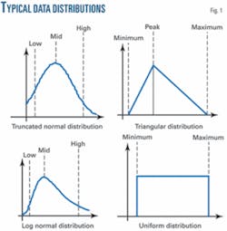
The conditions surrounding the particular variable, and therefore specific to the parameter in question, shape the distribution and the definition of the low, mid, and high values (or average and standard deviation of the values).
Typical distributions include:
- Truncated normal (used for general corrosion distribution in accordance with DNV G1011).
- Log normal (used for pitting corrosion defects in accordance with DNV G1011).
An analysis of actual operational data normally determines other distributions, examples include:
- Triangular (used for inhibitor effectiveness and availability; based on typical operational variations).
- Uniform (used for pressure; this is based on typical operating variations where a wide range of pressures with no discernable pattern occurs).
- Minimum extreme (used for temperature under rapid cooling pipeline conditions).
Wherever possible, distribution should be the best fit obtained from the actual operational data. In situations where the data are insufficient to allow analysis, or where operational experience is limited, it is recommended that a triangular distribution be used for all unknown parameters.
Fig. 1 shows some examples of these distributions.
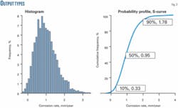
A Monte Carlo simulation can embed the distributions into a standard corrosion rate or metal-loss calculation. The simulation calculates multiple scenarios of a model by repeatedly sampling values from the probability distributions for the different uncertain variables. A single trial carries a randomly selected value from each of the defined ranges through the model to produce an output. Multiple passes are carried out (typically 1,000-10,000), defining a range of possible outcomes. Either a histogram or a probability profile (also known as a cumulative probability curve or S-curve) represent the results (Fig. 2).
A histogram displays all the outcomes along the X-axis and the probability (frequency) of occurrence along the Y-axis. It divides the X-axis into a suitable number of equal intervals, allowing the shape of the range of outcomes to be visualized and the symmetry and peaks in the distribution to be seen.
The S-curve shows the likelihood or probability of reaching certain values. The Y-axis displays the cumulative frequency as a function of the output values along the X-axis. A steep and narrow S-curve shows less uncertainty, while a wide and long S-curve shows more uncertainty in the variables.
Case Study 1
Unexpected corrosion prompted an internal corrosion threat analysis on a pipeline carrying crude oil from an offshore platform to onshore processing for a client in the Middle East. The analysis assessed the effect of accelerating corrosion-mitigation measures.
The pipeline, commissioned in 1999, is operation-critical as it carries the operator’s total production from a relatively small un-manned offshore production platform to onshore processing facilities. Design of the pipeline used the field’s expected 20-year production life.
The pipeline operated without inhibition before commissioning of the chemical injection facilities. Injection of corrosion inhibitor began at a reduced rate as compared with original target dose rates due to problems with injection pump capacity and limited control on management of the inhibition processes. Inspection of the accessible offshore production manifold sections showed that corrosion was occurring in the manifold sections of three producing wells.
Modeling sought to:
- Determine whether any damage to date had a major effect on the 20-year design life of the main oil line.
- Carry out an assessment of the effect on the probability of failure of the pipeline of implementing an improved chemical injection program.
- Carry out an assessment of the effect on the probability of failure of the installation of pig traps now and in future to enable routine cleaning pigs to be run, removing debris from the pipeline and improving the effectiveness of chemical inhibition.
The operator wanted to assess the effect of deferring the costs of implementing the programs against the enhanced risk of failure.
Threat assessment
Review of operating conditions, fluid chemistry, inspection reports, and pulled tubing surveys confirmed the main corrosion threat to be pitting corrosion due to dissolved CO2 and H2S, leading to formation of iron sulfide films. Inhibitor dosage records revealed historical under-dosing of product against target concentrations, although there was good correlation with iron count data that the inhibitor was effective when dosages were achieved.
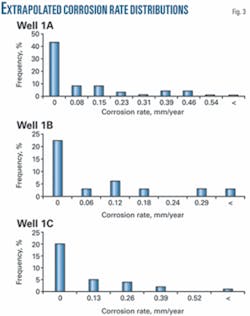
Inspection data taken from manifold pipework at the pipeline inlet generated a statistical distribution of likely corrosion rates. Fig. 3 shows examples of the range of calculated corrosion rates from inspection data.
Operating history
Analysis considered two distinct periods of historical operation:
- Period 1: From the time of commissioning (September 1999) to December 2001, during which time the line operated with no corrosion inhibition.
- Period 2: From December 2001 to January 2004, during which partial inhibition was in place.
Future scenarios
Analysis also evaluated four potential future operating scenarios:
- Scenario 1: Continued operation with no pigging and the current inhibitor regime.
- Scenario 2: No pigging but implementation of an improved corrosion inhibitor program.
- Scenario 3: Pigging in 2008 followed by an improved inhibition program.
- Scenario 4: Pigging in 2004 followed by an improved inhibition program.
The time taken to reach minimum allowable wall thickness due to corrosion, starting from nominal wall thickness at the time of construction, defined pipeline failure for this analysis. Monte Carlo uncertainty modeling evaluated the effect of each scenario on the projected time to failure using the iDecide software package.
Historic operating conditions resulted in the internal surface of the pipe being heavily scaled, with a high accumulation of deposits. Simply increasing the availability of the corrosion inhibitor, therefore, would likely not result in the same increase in life extension expected from a highly effective inhibition program on a clean pipe surface.
Routine maintenance pigging will increase inhibitor efficiency, but its effects are not easily quantified. The uncertainty modeling approach, however, allowed quantification of this difference in life extension.
Analysis considered the following factors:
- Inhibitor efficiencies in terms of mitigating both general corrosion and pitting corrosion in a sour system.
- Realistic, achievable potential inhibitor availabilities and efficiencies from an optimized inhibition program applied to future operations.
- Improvements in inhibitor performance with regard to pitting corrosion, based on previous experience of inhibitor selection and inhibitor performance.
Table 1 shows the range of values taken for the different conditions, together with the type of distribution.
Results
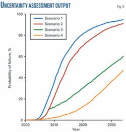
Fig. 4 shows results of the Monte Carlo assessment as cumulative probability curves (S-curves) for the probability of pipeline failure (defined as time to MAWT) for the four different scenarios. A clear difference in the likelihood of failure exists, creating an equally clear difference in the risk associated with the different operating scenarios. The additional inhibitor efficiency pigging would provide in mitigating future pitting corrosion sharply deferred the likelihood of failure-perforation.
It is also clear that simply improving the inhibition program, without pigging the line to address the build-up of deposits, has only a marginal benefit on the line’s longevity. By cleaning the line, pigging greatly improves the performance of the corrosion inhibitor at existing pits. In a system in which degradation is driven by localized corrosion, maximizing inhibitor efficiency has great benefits in deferring the potential time to failure.
Table 2 shows, even given the uncertain effect of pigging on inhibitor efficiency, modeling can still evaluate its potential effect on time to failure.
Enhanced inhibition alone only defers the time to 10% probability of failure by 3 years, while beginning routine pigging immediately defers it by 13 years. Deferment of 50% is again only 3 years for improved inhibition alone, increasing to 17 years with routine pigging commencing in 2008, but extending to 22 years by starting routine pigging immediately.
Simple inhibition, without regular cleaning, will almost certainly result in pipeline failure long before the design life of the pipeline.
While Fig. 4 and Table 2 clearly show the improvement in long-term integrity brought about by regular pigging, cost efficiency can also be identified by considering the effect of the additional operating costs for Scenarios 2, 3, and 4 as compared to Scenario 1 (maintaining the current inhibition program).
Cost estimates for an improved inhibitor program (covering higher dosage rates and improved availability) stood at an estimated $60,000/year; the cost of implementing a regular pigging operation (for the unmanned platforms) was estimated at $100,000/year; and the cost of a pipeline failure was estimated at $25 million.
Assuming a 5% interest rate allows calculation of the net present value, taking into account the operating costs each year as well as increased risk of failure. Table 3 shows the estimated net present value of the four different scenarios and relative costs over 10 years of operation.
Table 3 shows little benefit in simply adopting an improved inhibitor program, but significant benefit from incorporating routine pigging as soon as is practical.
Acknowledgment
The authors thank their coworkers for development of the overall procedure and the analysis of specific pipeline assessment.
Reference
- DNV-RP-G101, “Risk-based Inspection of Offshore Topsides Static Mechanical Equipment,” Det Norske Veritas, 2002.
The authors
Kirsten Oliver is business manager for corrosion and integrity work at the Intertek group’s CAPCIS Corrosion and Materials Consultancy. She has expertise in material degradation as it affects the water, oil and gas, and power industries. Before joining CAPCIS, Oliver worked as an operational corrosion engineer for Oceaneering, seconded to Shell, and in the research and development department of a UK water company. She received a bachelors of engineering degree with honors material science, University of Liverpool (1993) and a PhD (1996) in composite materials, also from the University of Liverpool. Oliver is a member of the Institute of Materials.
Gareth John works for the Intertek group as a senior corrosion consultant at CAPCIS. He specializes in corrosion management, corrosion control (in particular cathodic protection), and corrosion monitoring and testing. Gareth joined CAPCIS more than 27 years ago, following completion of his PhD (1979) in corrosion science at University of Manchester Institute of Science and Technology. He is a member of the Royal Society of Chemistry, an Institute of Corrosion fellow, and a NACE International certified corrosion specialist.


