PIPELINE FAILURE RATES-1: Method helps pool multisource data
The statistical uncertainty in the estimation of the average failure rate of a group of pipelines decreases as failures, km-years, or both increase. This fact has led to the tendency in pipeline reliability analyses to increase the number of km-years from which the failure data are pooled, reducing statistical uncertainty associated with estimating the failure rate.
This approach, however, is only valid if the uncertainty arising from the physical, environmental, and maintenance differences between pipeline systems is negligible.1
Oil and gas pipeline systems encompass many failure mechanisms, the most common being corrosion metal loss, third-party damage, geotechnical hazard, hydrogen-assisted and stress-corrosion cracking, and construction or material imperfections.2 These failure mechanisms can lead to ultimate failure modes, such as rupture and leakage.
Tolerance uncertainty describes the statistical errors that arise from merging inhomogeneous pipeline failure datasets. Pipeline failure-rate estimation, however, has consistently ignored tolerance uncertainty. A reliability methodology that allows estimating the pipeline population-failure rate together with the statistical and tolerance uncertainties associated with the estimate would yield more accurate results. A key element of this methodology should be the ability to establish whether the pipeline systems are similar enough to allow pooling of failure data across systems.
This article proposes such a methodology. This methodology holds particular utility when, rather than relying on average values, the failure rate needs to be estimated accurately from data gathered for multiple pipeline systems showing significant physical, environmental, and maintenance differences. It allows for addressing failure processes with constant or varying intensity and testing whether the pipeline systems are similar enough so that pooling failure data across them can reduce the statistical uncertainty in the failure rate estimation.
Current pipeline reliability analyses tend to increase the number of km-years from which the failure data are gathered with the purpose of reducing statistical uncertainty. This might lead pipeline operators to establish improper maintenance priorities due to the large tolerance uncertainty associated with pooling failure data across dissimilar pipeline systems. This article intends to raise awareness of this problem and provide pipeline reliability analysts with the methods to address it properly.
Part 1, presented here, offers the new methodology for estimating failure rates of a pipeline population from historical failure data pooled across pipeline systems based on the statistical methods for the reliability of repairable systems. Pipelines are repairable systems since, upon failure, they can be restored to operation by some repair process other than total replacement.3 4 Part 2 will outline and illustrate this methodology using real failure data compiled by the Office of Pipeline Data from oil and gas pipeline systems in southern Mexico and the US.
Basic definitions
This article treats pipelines as repairable systems. The term pipeline system refers to a group of pipelines that can be modeled by the same point stochastic process to describe the occurrence of failures in time. A pipeline system, therefore, is a repairable system with repairable subsystems (pipelines) that can all be described by the same process.
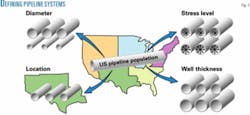
This allows assessment of tolerance uncertainty from system-to-system only when failure data are mixed to estimate a generic failure rate for the pipeline population. The totality of the pipeline systems used to carry out such estimation comprises a sample of the population under investigation. Fig. 1 illustrates some defining system variables for the US pipeline population.
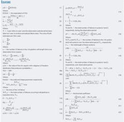
Equations 1 and 2 (see accompanying equation box) let N(t)be a random variable that defines the number of failures in the interval [0, t] in a pipeline system. The system rate of occurrence of failures at time (ROCOF), μ(t), and intensity function, λ(t), are shown by Equations 1 and 2, respectively.
This paper uses the term failure rate in the ROCOF sense, provided that the ROCOF and the intensity function are considered equal and that both are measures of the reliability of repairable systems. The time subinterval, Δt, is taken as 1 year; referring to the annualized failure rate of the pipeline system.
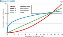
Mechanisms that do not depend on time and show a constant failure rate can be modeled with a homogeneous Poisson process (HPP) with constant intensity λ. Cases in which the system deteriorates or improves its reliability with time should use the non-homogeneous Poisson process (NHPP). Fig. 2 shows the trend of N(t) over service time for these reliability conditions.
null
Nonparametric estimate
Assume that a pipeline system has a total number of TexpLexp km-years; Texp and Lexp being the observation time interval (in years) and the total system length (in km), respectively. If the total number of failures is N(Texp) over the observed interval (time truncated case), then Equation 3 expresses the nonparametric estimate of the system failure rate.
On the other hand, focusing on the time evolution of λ rather than its mean value over Texp yields a simple nonparametric estimator of the system ROCOF (Equation 4).
Parametric estimate
If there are np pipelines in a system that can all be modeled by the same HPP, Equation 5 estimates the failure rate for the entire system.
In a time-truncated situation, when all pipelines have been observed over the same interval, ti = Texp, Equation 6 makes Equation 5 equal to Equation 3.
It is important to note, however, thatAccording to the HPP, the quantity 2 λ Texp has a chi-square distribution with 2N (Texp) degrees of freedom. Equation 7 provides a 100(1 - α)% confidence interval for λ.
Equation 7 predicts that the statistical uncertainty associated with predicting λ under the HPP model decreases when the number of failures or the number of km-years, or both increase.
Power law
Equations 8a and 8b model the time evolution of the expected number of system failures and the ROCOF for the power law process.
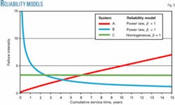
The shape parameter β determines whether the system deteriorates (β > 1), improves (β < 1), or remains the same (β = 1) over time. Fig. 3 shows the failure intensity function for the systems considered in Fig. 2.
If there are np pipelines in a system which can be all modeled by the same power law process with parameters β and θ and all pipeline failure data are time truncated at the same time Texp, Equation 9 shows the maximum likelihood estimate of β.
Equation 10 calculates the maximum likelihood estimate for parameter θ.
Equation 11 estimates the intensity function of the process in the pipeline system from the results of Equation 10.
The quantity 2N (Texp)β /Equation 13 yields a 100 (1 - α)% confidence interval at time t regarding failure rate.1
Before computing the pipeline system’s failure rate, it is important to check whether the system behaves, with respect to the evolution of the number of failures with time, as a homogeneous or a non-homogeneous Poisson process.
Truncated data require the statistic 2N (Texp)/This test behaves optimally if the alternative is that the failure process is a power law process with intensity function given by Equations 8a and 8b.3 4
Pooling data
When failure data are available from more than one pipeline system, the pooling of these data across systems must occur with caution. Several tests can help determine if the systems are dissimilar enough that the process parameters for each system should be estimated independently or if they are similar enough that their failure data can be merged.
The HPP assumption commonly uses the Fisher (F) test to determine similarity between failure datasets prior to merging. If the failure data of two pipeline systems are to be aggregated and the systems are assumed to be modeled by an HPP with identical failure rate, and the data are either failure or time-truncated, the null hypothesis that the λ’s are equal (H0: λ1 = λ2 ) can be tested against the two-sided alternative hypothesis Ha: λ1 ≠ λ2.
Equation 15 holds when the null hypothesis is true.
Accordingly, rejection of the hypothesis that both systems have identical failure rates occurs at chosen significance level, α, if F > Fa/2 (2N1, 2N2) or F < F1-α/2 (2N1, 2N2).
The opposite situation, where there is no evidence to reject the null hypothesis, allows for pooling of the failure datasets of the two systems. In this case, Equation 3 estimates the failure rate associated with the mixed data sets, while Equation 7 provides the estimate’s confidence bounds.
If the failure data of k pipeline systems need to be aggregated and the systems are assumed to be modeled by an HPP with identical failure rate, investigating whether the failure data from these systems can be mixed requires testing the null hypothesis H0: λ1 = λ2 = λ3 = ... λk against the alternative that at least one of the λ is different.
For both the failure and time-truncated cases, distribution of the following statistics, based on a likelihood ratio (LR), takes a roughly χ2 distribution with (k - 1) degrees of freedom (Equation 16).
The LR statistic provides a good approximation to the χ2 distribution for moderate to large Ni (Texp). For small values of Ni (Texp), the modification of this statistic provided by Equation 17 might increase the accuracy of the χ2 approximation.3
If the statistic LR (or LRM) is greater than the critical value ΧAs in the two-system case, Equations 3 and 7 estimate the failure rate and the confidence bound of the estimate, respectively.
According to the power-law process assumption, merging failure data of two pipeline systems involves two steps. The first is testing whether the shape parameters (β’s) estimated for both systems are identical and the second is testing if the failure rates of the systems are also identical.
The Fisher test compares the null hypothesis, H0: β1 = β2, with the two-sided alternative hypothesis, Ha: β1 ≠ β2. An accurate Equation 18 proves the null hypotheses true for the time-truncated case.
Either F < F1-α/2 (2N1, 2N2) or F > Fα/2 (2N1, 2N2) leads to a rejection of thehypothesis that the β’s estimated for both systems are identical.
The lack of a reason to reject the hypothesis that the estimated β’s are identical provides the basis for investigating whether the failure rates for the two systems are similar: testing the null hypothesis, H0: λ1 = λ2, against the alternative hypothesis Ha: λ1 > λ2. This process uses the approach proposed by Lee to test for equal failure rates (once the β’s have been proved to be identical).5
This approach gives the system with the longer observation period the number 1.5 The probability that the system experiences N1 (Texp) - 1 failures or less determines the probability that system 1 experiences N1 (Texp) or more failures over the observation period Texp. The total number of failures in the two systems, NT, and the sum of the logarithm of the failure times, S, condition these probabilities (Equation 19).5
Equation 19 says the larger theThe k pipelines case investigates the null hypothesis H0: β1 = β2 = ... = βk against the alternative hypothesis that at least two of the coefficients are different.3 Equation 20 provides a likelihood ratio statistic which can perform this investigation as a χ2 distribution with (k - 1) degrees of freedom.
Equation 9 calculates the estimatesRejecting the null hypothesis prohibits the failure data collected for the k systems from being merged. If there is no evidence to reject the null hypothesis, one can investigate if the failure rate λi of the k systems is similar. Testing the null hypothesis H0: λ1 = λ2 = ... = λk against the alternative hypothesis that at least two of the systems show different failure rates tests the equality of the λi. Equation 22 can perform this test.5
Equation 22 shows an Χ2 distribution with (k - 1) degrees of freedom when the total number of failures in the k systems over the observation time is large (N (Texp) ≥ 30). Once computed, the hypothesis that λ1 = λ2 = ... = λk can be rejected at a significant level, α, whenNot rejecting the hypothesis that the βi and λi’s are similar for the k systems allows the failure data to be pooled across these systems to produce a generic failure rate with a reduced statistical uncertainty.
Acknowledgments
The authors thank Hugo Huescas for gathering the failure data used in this work. They are also grateful to Petróleos Mexicanos (Pemex) for permission to publish these results.
References
- Fragola, J. R., “Reliability and risk analysis data base development: an historical perspective,” Reliability Engineering and System Safety, 51, pp.125-136, 1996.
- Kiefner, F., Mesloh, R. E., and Kiefner, B. A., “Analysis of DOT Reportable Incidents for Gas Transmission and Gathering System Pipelines: 1985 Through 1997,” Pipeline Research Council International, Catalogue No. L51830E, 2001.
- Rigdon, S. E., and Basu, A.P., Statistical methods for the reliability of repairable systems, New York: John Wiley & Sons Inc., 2000.
- Harold, H., and Feingold, H., Repairable Systems Reliability: Modeling, Inference, Misconceptions and Their Causes, New York: Marcel Dekker Inc., 1984.
- Lee, L., “Comparing rates of several independent Weibull processes,” Technometrics, 22(3), pp 427-430, 1980.
Based on presentation to the International Pipeline Conference, Calgary, Sept. 25-29, 2006.
The authors
Francisco Caleyo ([email protected]) is an associate professor at Instituto Politécnico Nacional de México (IPN). He heads a research team involved with the application of structural reliability analysis on onshore and offshore pipelines at the Centro de Investigación y Desarrollo de Integridad Mecánica (CIDIM) of the IPN. He holds a BSc in physics and an MSc in materials science from Universidad de La Habana and a PhD in materials science from Universidad Autónoma del Estado de México.
Lester Alfonso ([email protected]) is an assistant professor of Universidad Autónoma de la Ciudad de México. As a research professor at the CIDIM of the IPN, he develops numerical methods aimed at analyzing pipeline reliability and risk. He holds a BSc and an MSc in mathematical physics from Moscow State University and a PhD in atmospheric sciences from Universidad Nacional Autónoma de México.
Juan Alcántara is a member of the CIDIM of the IPN. He holds a BSc in physical metallurgy from IPN and is currently pursuing an MSc at the IPN in topics related to pipeline integrity and reliability analysis.
José Manuel Hallen ([email protected]) is a full professor at the IPN and heads the CIDIM, which has service contracts with Pemex to conduct mechanical integrity and risk analyses of onshore and offshore pipelines. He holds a BSc and an MSc in physical metallurgy from IPN and a PhD in physical metallurgy from the University of Montreal.
Francisco Fernández-Lagos is a senior pipeline integrity specialist with more than 20-years’ experience at Pemex. He currently works as pipeline integrity manager at the Gerencia de la Coordinación Técnica Operativa (GCTO) of Pemex. He holds a BSE in electrical control from Universidad Veracruzana and an MSc in pipeline management engineering from Universidad de las Americas.
Hugo Chow ([email protected]) is a senior pipeline integrity specialist with more than 20-years experience at Pemex. He currently works as pipeline integrity vice-manager at GCTO. He holds a BSE in electrical control from Instituto Tecnololgico de Ciudad Madero and an MSc in pipeline management engineering from Universidad de las Americas.


