Lean Energy Management-9: Boosting, support vector machines and reinforcement learning in computer-aided lean management
In past articles in this series, we have been outlining an approach to computer-aided lean management (CALM). CALM is coming of age now because the computational capabilities to realize it in practice are just emerging.
For the first time, real-time business is truly possible in the upstream oil and gas industry. Here we describe another essential piece of CALM, computational machine learning (ML). ML provides the essential CALM linkage between real-time data streams, information-to-knowledge conversion, and automated decision support.
The natural progression in lean energy management (LEM) is from understanding data, to modeling the enterprise, and then to the addition of new computational technologies that learn from successes and failures. Continuous improvement is not only possible but enforceable using software.
We know the energy industry has enough data and modeling capabilities to evolve to this new lean and efficient frontier.
Whenever an event happens, such as the Aug. 14, 2003, blackout in the northeastern US, or the sinking of the deepwater oil production vessel off Brazil in 2001, study teams are set up that quickly review all incoming data, model the system response, identify exactly what went wrong, where and when, and develop a set of actions and policy changes to prevent the event from happening again.
In other words, we always seem to be able to find the failures after the fact and identify what needs to be done to fix the procedures and policies that went wrong. Why can’t we use the same data to prevent the “train wrecks” in the first place? LEM provides the infrastructure necessary to accomplish that goal.
LEM requires that this data analysis, modeling, and performance evaluation be done all day, every day. Only then can the system be empowered to continuously learn in order to improve performance.
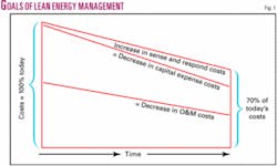
The increased costs for migrating to this new “sense and respond” operational framework are easily offset by subsequent decreases in capex and O&M costs that have been documented in industry after industry (Fig. 1).
Add computational ML to the data analysis loop and you have what is termed an adaptive aiding system. A car navigation system is one common example of this. The car’s GPS system learns when you make a wrong turn and immediately re-computes a new recommended course correction.
It is the feedback loop of such LEM systems that contains the newest and most unfamiliar computational learning aids, so we need to step through the progression of technological complexity in more detail.
Actions taken based upon information coming in are objectively scored, and the metrics that measure the effectiveness of those actions then provide the feedback loop that allows the computer to learn. In other words, once software infrastructure is in place, the continual recycling between decisions and scoring of success or failure throughout the organization are used to guide operators to take the best future actions.
Computational learning
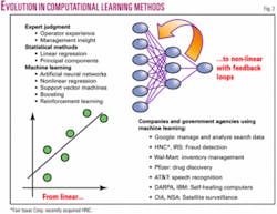
Computational or ML has proved effective at predicting the future in many industries other than energy (c.f. www.stat.berkeley.edu/users/breiman). Luckily, the field of computational ML has recently extended the range of methods available for deriving predictions of future performance (Fig. 2).
Examples of successful computational learning abound. It is now used to interpret user queries in Microsoft Windows and to choose web advertisements tailored to user interests in Google and Amazon.com, for example. In aerospace, computational ML has driven the progression from flight simulators that train pilots to computers that fly the plane completely on their own and soon to the newest Unmanned Combat Air Vehicles like the X-45 that can dogfight with the best “Top Gun” pilots.
Other successes are found in the progression from speech recognition to synthetic conversation and now to synthesizers of journalism itself (www.cs.columbia.edu/nlp/newsblaster).
In the automotive industry, there are new navigational aids that can park a car, not just assist the driver. Examples of other successful uses of ML are given in the online appendix for this article (www.ogjonline.com).
ML methods effectively combine many sources of information to derive predictions of future outcomes from past performance. Individually, each source may only be weakly associated with something that we want to predict, but by combining attributes, we can create a strong aggregate predictor.
Additional advantages of computational ML over traditional statistical methods include the ability to take account of redundancy among the sources of evidence in order to minimize the number of attributes that need to be monitored for real-time assessment and prediction.
Suppose we want to classify a data stream into like-performing characteristics. If we have a lot of data about what we want to predict, we will need a complex function that uses almost everything we know about the object, and still we will have imperfect accuracy.
To accomplish this, we must start with some already-classified example data we can use to train an ML system. ML techniques allow the system to find good classifying and ranking functions in a reasonable amount of computer time for even the largest of data sets. Although there are a wide variety of ML approaches, they have common features:
1. Adding more data over time improves accuracy. With just a few points, the ML algorithms can make an educated guess. As the number of data points rises, the confidence and precision of the results rises, also.
2. Each ML technique prefers some explanations of the data over others, all else being equal. This is called an “inductive bias.” Different ML approaches have different biases.
ML techniques mathematically combine the results of computations that produce a score for each object reflecting the estimation of its likelihood of doing something, like failing, from an evaluation of all the variables of the data for that object.
Those with the highest scores may be viewed as being predicted to fail soon. The scores can be sorted, resulting in a priority order ranking for taking preventive actions among many similar objects. Which compressor in a large production facility to overhaul next is a common example.
The data we wish to analyze will always have many dimensions-each dimension is an attribute of the data. For instance a compressor has a large number of attributes, such as its age, what it is used for, its load, its configuration, etc. Each object analyzed by an ML algorithm is described by a large vector of these data points.
For example, compressor #433 has an age of 20 years; its location is 40s field, its peak load to rating is 80%; ... etc. If there are only two or three attributes per data point, we can view each reading as a point on either a plane or in three-dimensional space. We will usually have many more attributes than that, and thus be working with many dimensions.
High-dimensional mathematics works in a similar way to the math of two and three dimensions, even though our visual intuition fails. The techniques described below can be extended to thousands or even hundreds of thousands of dimensions. Further, special algorithmic techniques have been devised to make the larger dimensionality problems manageable.
Below, we describe the sophisticated mathematical approaches to ML in the simplest two and three-dimensional context so they can be easily understood. Among the most basic problems attacked by ML is learning how to sort items into classes. The same techniques can then be expanded from classification to rankings.
For instance, ML can begin by classifying which compressors are at extreme risk and which are not, at significant risk or not, at moderate risk or not, etc., and then the data can be used again to calculate a ranking of the risk of imminent failure for every compressor in the inventory.
Modern ML methods called support vector machines (SVMs) and boosting have largely replaced earlier methods such as the so-called artificial neural networks (ANNs), based on a crude model of neurons.
ANNs and other early ML methods are still widely used in the oil and gas industry. The modern methods have significant advantages over earlier ones. For example, ANNs require extensive engineering-by-hand, both in deciding the number and arrangement of neural units and in transforming data to an appropriate form for inputting to the ANN.
ANNs have been replaced in the financial, medical, aerospace, and consumer marketing worlds by SVMs and boosting because the new techniques use data as is and require minimal hand-engineering. Unlike ANNs, both SVMs and boosting can deal efficiently with data inputs that have very large numbers of attributes.
Most importantly, there are mathematical proofs that guarantee that SVMs and boosting will work well under specific circumstances, whereas ANNs are dependent on initial conditions, and can converge to solutions that are far from optimal. Details and web links to more information on ML are in the online appendix.
Support vector machines
SVMs were developed under a formal framework of ML called statistical learning theory (http://en.wikipedia.org/wiki/Vapnik_Chervonenkis_theory).
SVMs look at the whole data set and try to figure out where to optimally place category boundaries that separate different classes. In three-dimensional space, such a boundary might look like a plane, splitting the space into two parts.
An example of a category might be whether or not a compressor is in imminent danger of failure. The SVM algorithm computes the precise location of the boundary-called a “hyperplane”-in the multidimensional space.
By focusing on the points nearest the boundary, which are called “support vectors,” SVMs define the location of the plane that separates the points representing, in our running example, compressors that are safe from those that are in imminent danger of failure. SVMs work even when the members of the classes do not form distinct clusters.
One of the simplest methods for classification is to:
• View a training dataset as points, where the position of each point is determined by the values of its attributes within a multidimensional space.
• Use SVMs to find a plane with the property that members of one class lie on one side and members of the other class lie on the other side of the plane.
• Use the hyperplane derived from the training subset of the data to predict the class of an additional subset of the data held out for testing.
• After validation, the hyperplane is used to predict that future data is of the same class as those in the training set if it falls on the same side of the hyperplane.
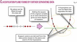
Finding a hyperplane that separates two classes is fairly easy as long as one exists. However, in many real-world cases, categories cannot be separated by a hyperplane (Fig. 4). In SVMs, extra variables are computed from the original attributes to further separate the data so a classification plane can be found.
For example, two categories that can’t be separated with a simple line in one dimension can be separated if we convert them into two-dimensional space by adding an extra variable that is the square of the original variable (Fig. 3). The data can now be separated by a hyperplane.
The breakthrough with SVMs was the discovery of how to compute a large number of variables, embed all that data into very high-dimensional space, and find the hyperplane effectively and efficiently.
Another important aspect of SVMs is that the hyperplane is chosen so that it not only correctly separates and classifies the training data but ensures that all data points are as far from the boundaries of the hyperplane as possible.
Avoiding overdependence on borderline cases protects against “overfitting,” a dangerous condition that produces “false positives” because the ML algorithm’s output has captured insignificant details of the training data rather than useful broader trends. We might then conduct preventive maintenance on the wrong compressor in our running example.
Boosting
All companies struggle within limited O&M budgets to deploy enough information sensors to make preventive maintenance predictions, so it is critical to determine what attributes are really needed versus those that are less useful.
An ML technique called “boosting” is especially good at identifying the smallest subset of attributes that are predictive among a large number of variables. Boosting often leads to more accurate predictions than SVMs, as well.
Boosting algorithms seek to combine alternative ways of looking at data by identifying views that complement one another. Boosting algorithms combine a number of simpler classification rules that are based on narrower considerations into a highly accurate aggregate rule.
Each of the simple rules combined by boosting algorithms classifies an object (such as a compressor) based on how the value of a single attribute of that object compares to some threshold.
An example of such a rule is that anyone in a crowd is a basketball player if his height is above 7 ft. While this rule is weak because it makes many errors, it is much better than a rule that predicts entirely randomly.
Boosting algorithms work by finding a collection of simpler classifiers such as these and then combining them using voting. Each voter is assigned a weight by how well it does in improving classification performance, and the aggregate classification for an object is obtained by summing the total weights of all the classifiers voting for the different possibilities.
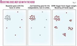
Voting increases reliability. If each voter is right 75% of the time, taking a majority vote of three voters will be right 84% of the time, five voters 90%, seven voters 92%, and so on. However, this only works if the voters are independent in a statistical sense. If there’s a herd of voters that tends to vote the same way, right or wrong, it will skew the results, roughly as if there were fewer voters.
Boosting algorithms try to only pick a single representative voter from each herd: undemocratic, but effective. In general, boosting tries to select a group of voters based on two competing goals: choosing voters that are individually pretty good, and choosing voters that independently complement one another as sources of evidence of the correct class of a typical object.
In the following diagrams, the points in the left and center represent voters (not data), and the distance between voters corresponds to the extent of similarity in their behavior (Fig. 4).
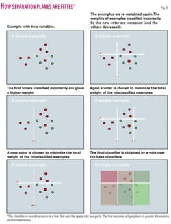
The series of diagrams in Fig. 5 illustrates the way the separation planes are fitted. The simple example is run for only three rounds on only two variables. In actual usage boosting is usually run for thousands of rounds and on much larger datasets. Boosting adds an additional classifier to the list for each round.
Before a given round, the examples are re-weighted to assign more importance to those that have been incorrectly classified by previously chosen classifiers. A new classifier is then chosen to minimize the total weight of the examples that it misclassifies. Thus, boosting looks for succeeding classifiers that make errors in different places than the others, and thus minimizing the errors.
In LEM, we use the ML tools that best fits each problem. We try several, and usually one will work better on some portions of the data than the others.
Our purpose in classifying is to gain fundamental understanding of the relationships between cause and effect among the many attributes contributing to the performance of each object. LEM can then manage many objects as integrated components of a larger system.
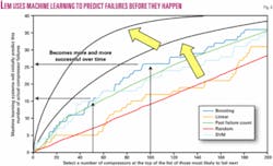
Consider the real-life example in Fig. 6. A good initial predictor can be derived by just looking at the number of past failures on each component (green curve), but nothing more is understood about cause and effect from an analysis of only this one variable.
If in addition, we apply both SVM and boosting, we gain insights into how the many attributes contribute to failure beyond just whether the component failed in the past or not. SVMs have an inductive bias towards weighing variables equally. In contrast, the inductive bias of boosting penalizes members of what appear to be “herds.”
SVMs often produce accurate predictions, but it is frequently difficult to get deeper intuition from them. In other words, SVM classifiers are often “black boxes.” Some insights may be possible if there are very few support vectors, but the number of support vectors rises rapidly with the amount of input data and the noisiness of the data.
Boosting has a better chance of giving actionable results, and it is particularly good at identifying the hidden relevance of more subtle attributes-an important benefit when looking for what is important to measure for preventive maintenance programs.
The above has described only static variables that do not change over time. ML analysis of the sequence of changes over time of dynamic variables is an important additional determinant for root cause analysis in LEM.
Magnitude and rate of change of the variables can be used to derive the characteristics leading up to failure of a group of objects so that precursors can be recognized for the overall system.
For compressor failure, for example, accumulated cycles of load can be counted and added as an attribute. Such dynamic variables are important in fields such as aerospace, where airplane takeoff and landing cycles are more critical predictors of equipment failure than hours in the air.
As these dynamic, time varying attributes are added to the ML analysis, new solution planes can be recalculated every time a new data update occurs and the differences between past solutions analyzed. Over time, the results migrate from prediction to explanation, and the feedback continues to improve prediction as the system learns how to optimize itself.
Reinforcement learning
Why go to all the added trouble required for ML?
Haven’t we been moderately successful managing our operations using policies and manuals derived from years of personal experience?
It’s because ML forces us to quantify the learning into models. Output from the SVMs and boosting algorithms can become the input into a class of ML algorithms that seek to derive the best possible control policy, whether for a plant, an oil and gas field, or for an entire organization or business unit.
One promising ML technique, called reinforcement learning (RL), is a method for optimizing decisions under uncertainty and over time, making it a powerful computer support tool for operators and managers. Its practical application is just emerging because the necessary real-time infrastructure is finally being built in the industry. Also, new ways to scale RL to problems with thousands of variables have only recently become available.
Suppose we have a number of states (situations), and actions must be taken by operators to move from the bad to good states. A small subset of the states will give a reward if entered. RL finds an optimal policy, i.e., situation-dependent action sequence, that results in the maximum long-term reward. RL is how the insights and predictions from SVMs and boosting are acted upon by the LEM organization.
A successful application of RL will result in a continuously updated decision support system for operational personnel, but only if there is a feedback loop established that allows the algorithm to learn from the rewards the organization receives from taking these actions.
In LEM terms, an “action driver” suggests what should be done in a specific situation. It must be attached to an “action tracker” that follows the results of that action and scores them based on whether or not they improved the state of the organization.
The rewards for successful actions are then used to reinforce the learning within the RL algorithm so it will know even better the policy that dictates the correct actions for the next similar situation that arises. In this way, the same mistakes are not allowed to be repeated by the organization.
An example for ultradeepwater operations might have as actions whether to switch a set of additional subsea separators into the flow lines over the course of a day’s production cycle. In the financial arena, the actions might be the choice of whether to store the oil onboard or sell into the pipeline at that particular time and price (real options). Executing the specific sequence of actions in a policy in successive time frames gives a recommended schedule (called a trajectory in RL).
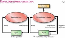
RL and LEM make a natural pairing. RL lets an enterprise explore and evaluate its ever-changing options as they arise. RL accomplishes this by using both real-time feedback loops and simulation models (Fig. 7).
RL maps from states to actions in order to maximize the numeric reward signal. The RL system is not told which actions to take, as with most forms of ML, but instead it must discover which actions yield the most reward by sampling the possible choices.
In the most interesting and challenging cases, actions will affect not only the immediate reward but also the next situation and beyond that all subsequent rewards. RL chooses these best operational actions using techniques similar to the dynamic programming method of real options valuation, with future rewards appropriately “discounted.”
RL methods have a number of features that are useful for LEM applications:
• RL does not make any strong assumptions about what system variables most influence the system’s performance. In particular, RL can cope with partial information and with both nonlinear and uncertain behavior. RL can therefore be applied to many types of control schemes in many different industries.
• RL uses closed-loop control laws that have been proved theoretically to be robust. This is important when the real system is facing situations that were not accounted for in simulation models of possible contingencies.
• RL learns continuously and adapts to changing operating conditions and system dynamics, making RL excellent for adaptive control.
Dynamic programming
RL is computationally difficult because the learning system must test many actions and then be told which of these actions were good or bad within an overall result through the action tracker.
For example, RL autopilot programs being developed to control an unmanned combat air vehicle (UCAV) are told not to crash. The RL algorithm must make many decisions per second, and then, after acting on thousands of decisions, the aircraft might crash anyway.
What specifically should the next UCAV learn from the last crash? Which of the many component actions, or chains of actions, were responsible for the crash? Assigning credit (or blame) to individual actions is the main problem that makes RL difficult.
A calculation technique known as dynamic programming (DP) makes the complex mathematics needed to solve this RL identification problem feasible. Finding a DP solution involves computing many intermediate results, each built from lower level results, over and over. DP calculates each intermediate result only once, and then it stores and reuses them each next time they are needed.
Even this technique is not scalable to many real-world problems because of the so-called “curse of dimensionality.” The computation required, even with DP, increases exponentially with the number of variables considered. In such cases, approximate DP methods have been developed to reduce the dimensions of the problem.
ML methods such as boosting and SVMs are used for approximate DP, although scaling RL to the number of inputs in real-time control is still a challenge. However, new methods to deal with thousands of variables are now available from research that has shown the commonality between real option valuation, optimal stochastic control, and reinforcement learning.
Pub/sub
In the near future, there will be two-way sensors on critical components throughout most business enterprises.
The data will drive a number of analysis engines evaluating large subsets of the sensors to determine real-time system decisions. A publish/subscribe system is the management layer that makes sure that each outgoing message goes to right place at the right time via secure pipes.
Publishers just emit data. Subscribers just describe what interests them. The publish/subscribe system ensures that subscribers receive all the relevant data that they need to optimize their individual decisions for peak performance of the overall system.
Combine all this, and LEM has the foundation for a pervasive RL model that can both provide operational decision support and plan for optimal performance under uncertainty far into the future. Everything from preventive maintenance to strategic planning and policy can be modeled with the RL system.
LEM is developing an ultimate RL model for the enterprise that will have predictive models for every key component. These, in turn, will be connected to models for each critical subsection, which in turn will be connected to network models, to districtwide models, and to regional and eventually to models of the surrounding environment critical to success beyond the company.
At every stage, the models will be constructed based upon SVMs, boosting, RL and other ML evaluations of what critical parameters of performance of each subsystem need to be monitored and modeled. In that way, only those key components will need to be instrumented for real-time control.
A pub/sub network is then set up to connect the information and learning loops amongst the models. Ultimately, the organization ends up with a unified model of its entire enterprise that is continuously and simultaneously optimizing financial and operational performance.
In industry after industry, the creation of that unified, enterprisewide model has proved to be the basic requirement for moving into a lean management future. Real-time business is the reason for computing the optimal financial and operational performance of an enterprise.
At Columbia University, we are using this approximate DP technique to solve both the RL and real option valuation problems with the same algorithm, simultaneously, as part of our Martingale Stochastic Controller.
The Martingale controller computes a solution that guarantees the maximum return from the integrated set of financial and operational decisions and will be the subject of the next installment of this continuing series on lean energy management. ✦
Bibliography
Anderson, R.N., and Boulanger, A.,“4-D Command-and-Control,” American Oil & Gas Reporter, 1998
Bertsekas, D.P., and Tsitsiklis, J.N., “Neuro-Dynamic Programming,” Athena Scientific, 1996.
Bellman, R.E., “Dynamic Programming,” Princeton University Press, Princeton, NJ, 1957..
Bellman, R.E., “A Markov decision process,” Journal of Mathematical Mech., Vol. 6, 1957, pp. 679-684.
Fernandez, Fernando, and Parker, Lynne E., “Learning in Large Cooperative Multi-Robot Domains,” International Journal of Robotics and Automation, special issue on computational intelligence techniques in cooperative robots, Vol. 16, No. 4, 2001, pp. 217-226.
Gadaleta, S., and Dangelmayr, G., “Reinforcement learning chaos control using value sensitive vector-quantization,” proc. International Joint Conference on Neural Networks, July 15-19, 2001, IEEE Catalog No. 0-7803-7044-9, ISSN 1098-7576, Vol. 2, pp. 996-1,001.
Gamba, Andrea, “Real Options Valuation: A Monte Carlo Simulation Approach,” Faculty of Management, University of Calgary, WP No. 2002/3; EFA 2002 Berlin Meetings Presented Paper, Mar. 6, 2002.
Kaelbling, Leslie, Littman, Michael L., and Moore, Andrew W., “Reinforcement Learning: A survey,” Journal of Artificial Intelligence Research, Vol. 4, 1996, pp 237-285.
Lau, H.Y.K, Mak, K.L., and Lee, I.S.K., “Adaptive Vector Quantization for Reinforcement Learning,” Proc. 15th World Congress of International Federation of Automatic Control, Barcelona, Spain, July 21-26, 2002.
Littman, Michael L., Nguyen, Thu, Hirsh, Haym, Fenson, Eitan M., and Howard, Richard, “Cost-Sensitive Fault Remediation for Autonomic Computing,” Workshop on AI and Autonomic Computing: Developing a Research Agenda for Self-Managing Computer Systems, 2003
Longstaff, F.A., and Schwartz, E.S., “Valuing American options by simulation: a simple least-squares approach,” Rev. Fin., Vol. 14, 2001, pp. 113-147.
Smart, William D., and Kaelbling, Leslie, “Practical Reinforcement Learning in Continuous Spaces,” proc. 17th international conference on Machine Learning 2000, pp. 903-910.
Sutton, R.S., and Barto, A.G., “Reinforcement Learning: An Introduction,” MIT Press, 1998.
Powell, W.B., and Van Roy, B., “Approximate dynamic programming for high-dimensional dynamic resource allocation problems,” in “Handbook of Learning and Approximate Dynamic Programming,” ed. by J. Si, A.G. Barto, W.B. Powell, and D. Wunsch, Wiley-IEEE Press, Hoboken, NJ, 2004, pp. 261-279.
Vollert, Alexander, “Stochastic control framework for real options in strategic valuation,” Birkhauser, 2002.
Werbos, P.J., “Approximate Dynamic Programming for Real-Time Control and Neural Modeling,” in White, D.A., and Sofge, D.A., eds., “Handbook of Intelligent Control,” Van Nostrand, New York, 1992.
The authors
Roger N. Anderson ([email protected]) is Doherty Senior Scholar at Lamont-Doherty Earth Observatory, Columbia University, Palisades, NY. He is also director of the Energy and the Environmental Research Center (EERC). His interests include marine geology, 4D seismic, borehole geophysics, portfolio management, real options, and lean management.
Albert Boulanger is senior computational scientist at the EERC at Lamont-Doherty. He has extensive experience in complex systems integration and expertise in providing intelligent reasoning components that interact with humans in large-scale systems. He integrates numerical, intelligent reasoning, human interface, and visualization components into seamless human-oriented systems.
Philip Gross is a PhD candidate at Columbia University doing research in the area of large-scale publish-subscribe networks and application of autonomic software principles to legacy distributed systems. He also works part time for Google. Prior to his graduate studies he was a systems consultant in the Netherlands for DEC and PTT Telecom.
Phil Long is a senior research scientist in the Center for Computational Learning Systems of Columbia University. He was on the computer science faculty at National University of Singapore in 1996-2001. In 2001, he joined the Genome Institute of Singapore before moving to Columbia in 2004. He has a PhD from the University of California at Santa Cruz and did postdoctoral studies at Graz University of Technology and Duke University.
David Waltz is director of the Center for Computational Learning Systems at Columbia University. Before coming to Columbia in 2003, he was president of the NEC Research Institute in Princeton, NJ, and earlier directed commercial applications research at Thinking Machines Corp. (1984-93) and held faculty positions at the University of Illinois (1973-84) and at Brandeis University (1984-93). He has a PhD from Massachusetts Insititute of Technology.
