Evaluating production potential of mature US oil, gas shale plays

Rafael Sandrea
IPC Petroleum Consultants Inc.
Tulsa
US oil supply has been on an unprecedented surge of 1.3 million b/d from an all-time low of 4.95 million b/d in 2008.
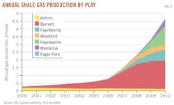
Current production of crude oil is 6.3 million b/d, the highest since 1997, and is expected to increase another 370,000 b/d in 2013. This exceptional growth in output was triggered mainly by major breakthroughs in production technology for tight oil resources headed by the Bakken, Eagle Ford, and Niobrara plays (Fig. 1). As recently as 5 years ago, we learned to efficiently drill horizontal wells with laterals as long as 8 miles and complete them with as many as 40 hydraulic fracs.

This modern technology has shaped a megatransformation in the US oil and gas industry. US natural gas supply has gone from shortage to abundance.
We can now access vast oil and gas resources that we have known to exist for decades but were impossible to recover because of their very low permeabilities (in the microdarcy range for tight oil and nanodarcy range for shale gas) and porosities that are a fraction of those of conventional reservoirs. By comparison, good conventional oil and gas reservoirs in the onshore US have permeabilities of 1-100 md and porosities of 10-15%.
Historically, horizontal drilling technology got its start in tight gas sands in the 1980s, subsequently moving into the almost impermeable (akin to concrete) shale gas plays at the end of the 1990s.
Specifically, the Barnett was the first shale gas play to be commercially developed. Modern horizontal drilling coupled with multistage fracing only began in the mid-2000s, and by 2008 there were 12,000 producing wells in the Barnett, of which two-thirds were horizontal and one-third vertical.
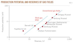
US marketed gas production was at a low of 46 bcf/day (bcfd) in September 2005 when shale gas output was only 1.4 bcfd. Since then, gas production has grown to 66 bcfd in 2011 and shale gas to about 20 bcfd, headed by the Haynesville (5.9 bcfd), Barnett (5.6 bcfd), and Fayetteville (3 bcfd), the three most developed of the shale gas plays (Fig. 2).
US consumption of gas is about 94% of domestic production, so supply is not as dependent on foreign producers as is the case for oil. The availability of large quantities of shale gas should enable the US to consume a predominantly domestic supply of gas for many years and produce more natural gas than it consumes.
The Energy Information Administration's Annual Energy Outlook 2012 projects US gas production to increase to 76 bcfd in 2035. Almost all of this increase is due to projected growth in shale gas production, to 37 bcfd by 2035.
On the US domestic crude oil front, the author's recent stochastic outlook indicates an upside output of 7.7 million b/d by 2025, of which half would come from tight oil plays. When potential output from natural gas liquids—mainly from shale gas plays—is factored in, total US liquids supply could reach 16 million b/d from 10 million b/d today.
Implicit in these upside scenarios for both oil and gas are several constraints of diverse nature, from environmental to policy issues, along with many technical challenges. This article addresses some of the major technical issues that affect estimates of two key parameters: the volume of recoverable oil or gas, and its production potential, which ultimately determine the value of the asset.
Both factors are physically interrelated and are indispensable for the planning of field infrastructure and takeaway capacity. They depend critically on field performance which is sparse given the short production history—barely 10 years—of shale plays.
Last summer, for example, the USGS (2011) sharply cut back the technically recoverable resource of the Marcellus play to 84 tcf from 410 tcf. The EIA subsequently upped it to 141 tcf in its 2012 Outlook. Production from the Marcellus barely started in 2008. In the past 3 years there have been similar fluctuations in recoverable oil and gas for several of the major shale plays.
An intrinsic characteristic of all shale plays is their extremely high initial decline rates (63%/year and more) with steep trends, a combination that is conducive to significant decreases in the recovery factor and a shorter economic field life. As a result, in the short production history of shale oil and gas there are already three mature plays: Barnett, Fayetteville, and Bakken (Elm Coulee). A thorough evaluation of their ample performance history will provide useful analogs for the many emerging plays. This is the main goal of this study.
Assessing US shale gas
Shale gas basics
Shale gas is natural gas that never migrated but remained trapped in the original source rock, adsorbed in the insoluble organic matter.
Gas shales are therefore both the source rock and the reservoir for the natural gas. They are characterized by ultralow permeabilities and the micropore spaces can barely accommodate the flow of tiny methane molecules. Gas production from hydraulically fractured shale is believed to come from both desorption and diffusion within the fracture network, in contrast to Darcy flow in conventional reservoirs. The mechanisms are still far from clear.
This complexity is why shale gas was the last major source of unconventionals (the others being tight gas and CBMs) to be developed. Shale gas production in effect took off in the mid-2000s, essentially after modern horizontal drilling and multistage fracing technology became widespread. And the Barnett was the pioneering shale play.
Produced shale gas is generally dry (less than 50 million bbl of NGL/tcf) although several plays have a liquid content of up to 125 million bbl/tcf, termed a rich gas. Barnett gas averages 87% methane with 83 million bbl/tcf, while the Fayetteville, Haynesville, and Marcellus have average methane contents of 87%, 95%, and 85%, respectively.
Shale gas resources are spread all over the US (Fig. 1) at depths varying between 1,000 ft and 13,500 ft. They are continuous, covering millions of acres, in contrast to discretely dispersed conventional oil and gas fields.
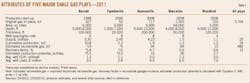
A good shale gas prospect is 300-600 ft thick. The five largest shale gas plays in the US are the Marcellus, Haynesville, Barnett, Woodford, and Fayetteville, with technically recoverable gas varying from 84 tcf for the Marcellus to 5 tcf for the Fayetteville. Table 1 summarizes general attributes of the plays.
EIA this year estimated that the US holds 3.7 quadrillion cu ft (qcf) of shale gas in-place of which 482 tcf are considered technically recoverable; barely 24 tcf have been produced. Worldwide, shale gas activity is still very low. Potential resources, excluding those in the US, are estimated by the EIA at roughly 5.6 qcf.
Decline analysis
The Barnett and Fayetteville are the only shale gas plays with sufficient production history to allow a comprehensive field decline analysis.
Production from each play has reached a volume roughly equivalent to the half-life of their recoverable reserves. Classical logistic decline analysis indicates estimated ultimate recovery of 19 tcf of gas for the Barnett and 5 tcf for the Fayetteville. The comparable estimates of technically recoverable resources, according to the recent EIA/AEO2012 report, are 26 tcf and 13 tcf, respectively.
Shale gas plays show unusually high field decline rates with very steep trends, a combination conducive to low EUR values, and consequently low recovery efficiencies.
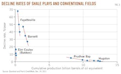
Fig. 3 gives a matchstick look at decline rate trends for the Barnett and Fayetteville, and for Hugoton, the largest conventional gas field in the US. The values shown on the graph refer to the last 3 years of production. The contrast between shale gas plays and conventional fields is astounding.
Keep in mind that extrapolating the decline rate trendline to rate = 0 gives the corresponding EUR value for the play. The steeper the trend, the smaller the EUR value and, consequently, the lower the recovery efficiency. Backward extrapolation of the trendline to the start of production (cumulative production = 0) gives the initial decline rate for the play, and all are evidently very high.
The abnormally high decline rates for shale gas have been recorded in producing wells from the very onset of field development. Recovery efficiencies calculated with these new decline EUR values for the Barnett and Fayetteville are 5.8% and 10%, respectively; this contrasts significantly with recovery efficiencies of 75-80% for conventional gas fields.
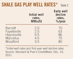
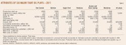
Table 2 gives initial well rates and first-year decline rates for large data sets of wells in the five major shale plays, as reported by Standard & Poor's Creditweek/Dec. 14, 2011. In general, average first-year well decline rates vary from 63% to 86% while initial well rates vary from 2 MMscfd for the Barnett to 9.5 MMscfd for the Haynesville.
About 75% of well EUR for the Barnett is produced by Year 5. Most wells have a commercial life of less than 15 years while EUR values refer to a 30-year life span.
The Haynesville is a unique shale play with extremely abnormal high initial well rates—about three times the average initial well rates of the four other major plays, with recorded well rates as high as 30 MMscfd—and abnormally high first-year well decline rates of 86%! This is a consequence of the fact that the Haynesville, the deepest of the major plays, is highly overpressured with pressure gradients in the range of 0.75-0.85 psi/ft.
By comparison, pressure gradients for the Barnett and Fayetteville are more in the range of 0.52 psi/ft. A normal field gradient is about 0.43 psi/ft. All considered, the recovery efficiency of the Haynesville is a low 4.7%.
The recovery efficiency for the five major plays averages 6.5% and ranges from 4.7% to 10% (Table 1). The EIA's estimate for all plays is 13% or nearly double. This would suggest that their estimate of 482 tcf of recoverable gas for the US should at best be 240 tcf based on present information.
It is worth mentioning that the USGS estimates of oil and gas in place for the different shale plays has proven to be dependable over time, the movable parameter being the recoverable oil and gas that defines recovery efficiency.
Production potential
It is a firmly established principle that reserves are the foundation of production potential and they follow a power law relationship. Fig. 4 shows the correlation of these two parameters for six conventional giant gas fields around the world.
Superposed on the graph are values for the Barnett and Fayetteville shale plays, the only two plays with adequate field data at this time. The shale gas plays are not conventional; their behavior indicates that their high peak production rates do not translate into a bigger (more reserves) field. By hypothesis, the shale gas plays should follow a similar power law relationship but parallel to that of the conventionals. We drew the trend line weighting the much larger Barnett. We would have to wait for data from future mature shale gas plays to fine-tune the specific trend.
The relationship for shale gas plays is
qpeak = 0.23 K1.0664 (1)
where qpeak is the production potential of the play with units of bcfd, and K is the size (reserves) of the play in tcf. This algorithm was used to estimate the production potential of the plays in Table 1, based on the current estimates of recoverable gas. Estimates of production potential are for the Marcellus 26 bcfd, the Haynesville 10 bcfd, and the Woodford 2.7 bcfd.
The equivalent relationship for conventional gas fields is
qpeak = 0.087 K1.0664 (2)
This shows that shale gas plays peak at rates 2.6 times those of conventional gas fields for the same size field. The similar exponents in both algorithms reflect the assumed parallel nature of the relationships. The correlation coefficient (r2) for Equation 2 is 0.994.
Assessing US tight oil plays
Tight oil basics
The Bakken has been the torch bearer of the shale oil revolution following the success of modern extraction technology applied to shale gas.
It is the largest commercial continuous oil accumulation in the world and currently accounts for almost two-thirds of all US shale oil production. The Bakken, Eagle Ford, and Niobrara are the three leading shale oil plays with 91% of total US shale oil output. These shale oil plays are now more commonly referred to as tight oil plays (Fig. 5).

In contrast to shale gas, which remained trapped in the original shale source rock, the Bakken, for instance, contains migrated oil trapped in siltstone and sandstone between layers of shale. The Eagle Ford's oil is trapped in carbonate rocks overlying the Eagle Ford shale from which it migrated.
Hence there is an important distinction (with shale gas) that affects the reservoir dynamics. In general, tight oil reservoirs are in close contact with their shale source, and induced fractures most likely extend into the shale providing some of the produced oil.
Tight oil reservoirs have higher permeabilities and porosities than their shale gas counterparts, in the range of 40 microdarcys with porosities around 5%, respectively. They are located at depths varying from 1,000 to 14,000 ft and area 10-3,000 ft thick. Table 3 summarizes the attributes of the top six major tight oil plays in the US.
Avalon and Bone Spring are two small plays with the Avalon sitting atop the Bone Spring formation. They are combined into a single unit in this study for lack of separate published data.
The EIA in 2012 estimated that the US holds 33 billion bbl of technically recoverable tight oil. The six major plays account for 31 billion bbl or 93% of the whole. Production history of tight oil plays starts in the early 2000s and is very limited; barely 585 million bbl have been produced so far from a national resource base estimated to hold over 3.5 trillion bbl. Likewise, worldwide activity can at best be described as embryonic.
Decline analysis
Elm Coulee field is the only tight oil play with ample production history to allow a comprehensive field decline analysis.
The field was discovered in eastern Montana in 2000 and produces from the Bakken. At its peak in 2006, Elm Coulee was producing 53,000 b/d from 350 wells or roughly 150 b/d/well. Today, output has dropped to 24,000 b/d, and cumulative production is 113 million bbl of 41° gravity, light sweet crude. Logistic decline analysis indicates an EUR of 130 million bbl, which corresponds to a 5.6% recovery factor.
A short review of some operational aspects of the field is appropriate since it is the best analog of the Bakken at this time. More than 600 wells have been drilled in the field with over 1,000 laterals, some as long as 10,000 ft. The Bakken interval ranges in thickness from 10 to 45 ft with porosities of 3% to 9% and permeabilities averaging 40 microdarcies. It is slightly overpressured with a gradient of 0.52 psi/ft.
Initial oil rates from the multilateral wells range from 200 to 1,900 b/d, compared with less than 100 b/d for vertical wells.
Fig. 2 gives a matchstick look at the decline rate trend for Elm Coulee. Observe the steepness of its decline rate trend, similar to that of the shale gas plays and very dissimilar to that of conventional oil fields represented here by giant Prudhoe Bay.
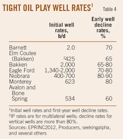
Table 4 gives initial well rates and first-year decline rates for Elm Coulee and the six major shale plays. With the exception of the Bakken that had its start in 2000, the other plays had starts after 2008. As such, the information on initial well rates and early well decline rates is limited because: 1) the number of wells drilled and producing is fewer and fragmented among many operators, and 2) information is slow in becoming public due to the intense economic activity associated with these oil plays.
We therefore opted to give the best range of data for the different parameters, in contrast to the average values given for the shale gas plays. Data for shale plays is very location sensitive; many well samples are required to establish statistically reliable values.
In general, first-year well decline rates are typically high for tight oil plays, varying from 65% to 90%, while initial well rates vary from 400 to 2,000 b/d for the Bakken and Eagle Ford. For a type well in the Bakken, almost half (46%) of its EUR is produced by Year 5; the other half to be produced over the following 25 years!
The Niobrara and Monterey are still under appraisal in specific areas as evidenced by their high well density: 8 and 12 wells/sq mile, respectively, vs. 2 for the Bakken (Table 3). For the sake of comparison, initial well decline rates for conventional oil field wells are in the range of 5-10%.
Regarding recovery efficiencies there are only two values available from field data. One, 5.6% that was established by decline analysis for Elm Coulee and 1.25% for the Bakken as a whole. This latter value is the result of an NDGS report released by the state of North Dakota in 2006; it is the value also used by the USGS in their assessments of other tight oil plays. Why this broad range of values?
As mentioned previously, shale and tight oil plays are continuous accumulations over extensive areas in contrast to conventional discrete oil fields that are geologically disconnected. In this respect, oil fields like Elm Coulee are better described as sweet spots that have better-quality matrix reservoir properties (permeabilities greater than 0.15 millidarcys and extra natural fractures) than the surrounding area in the play.
The recovery factor of 5.6% explicitly refers to the in-place volume of oil in the specific Elm Coulee sweet spot. When recovery is measured with reference to the entire active area surrounding the sweet spot, which includes productive and nonproductive areas, then the recovery factor drops considerably.
Sweet spots are randomly located within a play. A play may have good hydrocarbon potential but widespread success in locating sweet spots is the final determinant. The recovery factor cited in the NDGS report refers to the average over the active area. It is the appropriate approach for continuous resource-based deposits, and a recovery factor of 1-2% seems to be the best estimate to be used for other emerging tight oil plays at this time.
Production potential
Fig. 6 shows the correlation between production potential and recoverable oil (EUR) for five conventional giant oil fields from around the world.
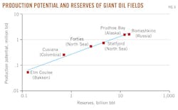
When the values for Elm Coulee field are included they fall perfectly on the trend. The resultant algorithm is
qpeak = 0.26 K0.7088 (3)
where qpeak is the production potential of the play with units of million barrels per day, and K is the size (reserves) of the play in billions of barrels. The correlation coefficient (r2) for Equation 3 is 0.993.
This relationship is pleasantly interesting since it confirms that tight oil reservoirs do follow the dynamics of the Darcy flow regime as do conventional oil reservoirs, an important contrast with shale gas reservoirs discussed previously.
As a side remark, tight gas sands do behave in a way physically similar to conventional gas reservoirs; however, their recovery factors are low, 6-10%.
The above algorithm was used to estimate the production potential of the major plays in Table 3, based on the current estimates of recoverable oil. Potential estimates for the Bakken are 815,000 b/d, Eagle Ford 565,000 b/d, and Avalon/Bone Spring 360,000 b/d. Niobrara's estimated potential is 1.03 million b/d, and Monterey's is 1.68 million b/d. These huge potentials are strong incentives to resolve the equally huge technical challenges that lie ahead in these two plays.
Summary results
An in-depth analysis was made of the production performance of the Barnett and Fayetteville shale gas plays and of Elm Coulee Bakken oil field.
These are the only existing mature fields of shale gas and tight oil resource plays, and the object was to establish field performance values of key parameters such as recoverable oil and gas and recovery efficiencies and, ultimately to develop algorithms that can provide a reliable estimate of production potential. This latter parameter is fundamental to the planning of production and take-away infrastructure, and finally determines the value of the asset.
Salient results of the study follow:
1. The top three producing shale gas plays: Haynesville, Barnett, and Fayetteville account for 70% of total US shale gas output, currently about 20 bcfd.
2. Shale gas plays show unusually high field decline rates with very steep trends, a combination conducive to low recovery efficiencies. The average recovery efficiency is about 7%, in contrast to recovery efficiencies of 75-80% for conventional gas fields. This suggests that the estimate of recoverable gas for all US shale plays should be near 240 tcf, or half of the 482 tcf now reported.
3. A power law relationship was developed that provides an estimate of production potential from knowledge of the volume of recoverable gas. Estimates of production potential for three major shale gas plays are: Marcellus 26 bcfd, Haynesville 10 bcfd, and Woodford 2.7 bcfd. The Barnett and Fayetteville are currently near their peaks. Shale gas plays peak at rates 2.6 times those of conventional gas fields of the same size.
4. The top three producing tight oil plays: Bakken, Eagle Ford, and Niobrara account for 90% of total US tight oil output, currently about 620,000 b/d.
5. Elm Coulee field is the only tight oil play with ample production history that allows a comprehensive field decline analysis. At this time, it is the best analogue of the Bakken, the biggest producer of all tight oil plays; the Bakken accounts for almost two thirds of total US tight oil output.
6. In some ways, tight oil and shale gas plays are similar. They are both extensive, exhibit high first-year well decline rates varying from 65% to 90%, and low recovery efficiencies averaged over the entire play: 7% for shale gas and 1-2% for tight oil. For 'sweet-spots' in the play such as Elm Coulee field, oil recoveries can reach 5-6%.
7. The power law relationship for estimating oil production potential is the same for both tight oil and conventional oil fields! The algorithm developed gives estimates of production potential for the Bakken of 815,000 b/d, Eagle Ford 565,000 b/d, and Avalon/Bone Spring 360,000 b/d. Estimates of potential for the Niobrara and Monterey tight oil plays are 1.03 million b/d and 1.68 million b/d, respectively. These two emerging plays have huge production potentials which certainly are strong incentives to resolve the equally huge technical challenges associated with their development.
Bibliography
"Texas Eagle Ford drilling, production spooling up," OGJ, Feb. 6, 2012, p. 46.
Redden, Jim, "Barnett shale: gas production rises despite lower rig count," World Oil, February 2012.
"Niobrara's true potential will take time to evaluate," Oil & Gas Financial Journal, February 2012.
Abraham, Kurt, "Fayetteville: remaining potential awaits higher prices," World Oil, March 2012.
Mason, James, "Bakken's maximum potential oil production rate explored," OGJ, Apr. 2, 2012, p. 76.
Sandrea, R., "US crude oil production potential: a stochastic outlook through 2030," PennEnergy Research Center, July 2012.
Sarg, Frederick, Sonnenberg, S.A., Batzle, M., and Prasad, M., "Bakken tight oil resource play—exploration model," National Energy Technology Laboratory/Colorado School of Mines project, Department of Energy Award DE-NT0005672, Nov. 11, 2011, available on line (geology.mines.edu/Bakken/.../Bakken%20Exploration%20Model.ppt).
Berman, A., and Pittinger, L., "US shale gas: less abundance, higher cost," The Oil Drum, Aug. 5, 2011.
Kaufman, Peter, "Maximizing potential of the Niobrara," Schlumberger, 2010.
"Review of emerging resources: US shale gas and shale oil plays," EIA/INTEK Inc., July 2011.
Verrastro, Frank, "The role of unconventional oil and gas: a new paradigm for energy," CSIS 16th Annual Washington Energy Policy Conference, Apr. 17, 2012.
Sonneberg, S., and Pramudito, A., "Petroleum geology of the giant Elm Coulee field, Williston basin," AAPG Bull., Vol. 93, Issue 9, 2009.
Sandrea, R., "Estimating new field production potential could assist in quantifying supply trends," OGJ, May 22, 2006.
Sandrea, R., "Equation aids early estimation of gas field production potential," OGJ, Feb. 9, 2009.
Mancini, Ernest, Li, Peng, Goddard, Donald, A., Ramirez, Victor, and Talukdar, Suhas C., "Mesozoic (Upper Jurassic-Lower Cretaceous) deep gas reservoir play, central and eastern Gulf Coastal Plain," AAPG Bull., Vol. 92, No. 3 (March 2008), pp. 283-308.
Fairhurst, Bill, Hanson, Mary, Reid, Frank, and Pieracacos, Nick, "WolfBone play evolution, southern Delaware basin: geologic concept modifications that have enhanced economic success," Search and Discovery Article No. 10412, posted June 18, 2012.
Sandrea, R., "World crude oil supply through 2030," PennEnergy Research Center, March 2012.
The author

Rafael Sandrea ([email protected]) is president of IPC Petroleum Consultants Inc., a Tulsa international petroleum consulting firm. He was formerly president and chief executive of ITS, a Caracas petroleum engineering firm he founded and directed for 30 years. He has a PhD in petroleum engineering from Penn State University.