PIPELINE INTEGRITY—2 (Conclusion): Model choice governs accuracy of corrosion predictions
Francisco Caleyo
Alma Valor
Victoria Venegas
Jose Hiram Espina Hernandez
Julio C. Velazquez
Jose Manuel Hallen
ESIQIE, Instituto Politecnico Nacional
Mexico City
Pipeline reliability analysis requires selection of a defect growth model that will accurately predict both the time evolution of corrosion defects and the probability of these defects' failure.
The first article in this series (OGJ, Oct. 1, 2012, p. 122) established the methodology for developing prediction models and examined each. This second, concluding article compares the models' performance before determining the Markov model as the model of choice for correct prediction of corrosion defect depth evolution and pipeline reliability.
The Markov model works well over a wide range of pipe ages and defect depths and can predict not only the time evolution of the entire defect depth population but also the evolution of the defects in subpopulations within different depth intervals.
It is also the only model that reproduces the time evolution of the corrosion defects from the depth data of the first inline inspection (ILI) and the value of corrosion rate ν estimated from two or more repeated ILIs, meaning no physical or chemical information is required to assess the actual corrosivity of the soil and its influence on the corrosion process to make relatively accurate estimations of the pipeline reliability over time.
It is also the only model capable of capturing the intrinsic, unavoidable stochastic nature of the corrosion process independent of the inspection tool's measurement errors or the initial defect depth distribution in the pipeline.
Reliability analysis
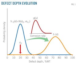
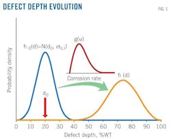
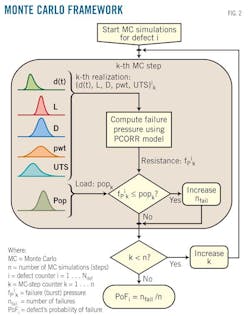
Figs. 1 and 2 depict the reliability framework used in this study.
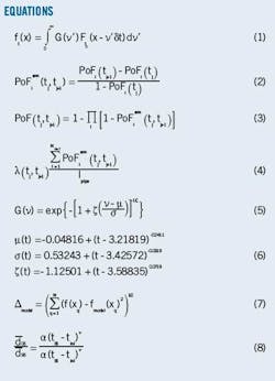
Fig. 1 shows how each depth in the ILI-measured pit depth distribution is affected by the inspection tool's random measurement errors during reliability assessment. A normal distribution with mean zero and standard deviation σILI of 8% pwt describes the uncertainties (OGJ, Sept. 13, 2004, p. 76). The resulting pit depth distribution for each defect located and sized by the first ILI, therefore, is also normal, with mean d0 and standard deviation σILI. This distribution occurs at the initial time, t0, and is evolved with use of each of the five corrosion rate models described in Part 1—represented by g(υ) (Fig. 1)—to obtain depth distribution, ft(d), of the defects at a future time, t (Equation 1 in the accompanying box).
Fig. 2 shows the next stage: the Monte Carlo framework. In each k-th Monte Carlo step, a vector with a realization of each one of the basic random variables, xik ={d,L,D,pwt, UTS}ik joins the PCORR model1 to calculate burst failure pressure (resistance), fiPk, associated with the i-th defect. The statistical variables are defect depth, d, and length, L, at time, t; pipe diameter, D, wall thickness, pwt, and tensile strength, UTS; and operation pressure, pop. Distributions of L, D, pwt, UTS, and pop are assumed normal, while defect depth distributions stem from the process illustrated in Fig. 1.
Researchers compared the calculated failure pressure for each defect with random values taken from the operation pressure (load) distribution. When popk ≥ fiPk, that is when the load is equal to or greater than the resistance, failure is assumed. Dividing the number of failures, nfail, by the total number, n, of Monte Carlo steps, produces an unbiased estimator of the probability of failure, PoFi, of the defect.
The above scheme repeats n times for each of the Ndef defects found in the ILI. The process, therefore, repeats n × Ndef times during the assessment. Researchers then repeat this procedure for several future times, tj, with time intervals of 1 year. Completing the calculations computes the probability of failure PoFi(tj) for each of the corrosion defects in the pipeline at each time, tj, computed.
Equation 2 calculates the conditional annual probability of failure, PoFiann of the i-th defect at tj. Given that the corrosion defects are independent, Equation 3 can calculate an upper bound of the annual probability of failure of the whole pipeline (OGJ, Jan. 6, 2003, p. 54). Equation 4 can calculate the pipeline's annual failure index, λ, at the end of the j-th year, lpipe being the pipeline length in kilometers. Given its definition, λ has units of failure of incidents/kilometer-year commonly expressed as 1/(km-yr).2
Models' performance
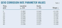
The five outlined CR models applied to the 1996-ILI data set analyzed a time span, dt = t-t0, of 10 years. The Markov model used an assumed characteristic pit initiation time of tini = 2.8 years, while t0 = 11 years, and t = 21 years. Equations 5 and 6 and Table 1 determined the CR distributions used in the TD-GEVD model for each year in the analysis interval, Year 11 to Year 21. The TI-GEVD model used the corrosion rate distribution predicted by Equations 5 and 6 for Year 11.
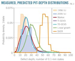
Fig. 3 shows the initial (1996-ILI) and final (2006-ILI) pit depth distributions on a probability density scale of the ILI measured and matched defects in the example pipeline. The defect depth is in units of 0.1 mm or Markov states. Initial depth distribution is represented in two ways: a histogram consisting of five states in each bin and a line running from state to state. The latter representation allows comparison with the SVCR. A histogram with five statewide bins displays the final ILI-measured depth distribution. Fig. 2 also shows the estimated pit depth distributions after a 10-year interval as predicted by the five CR models.
The SVCR model in Fig. 3 exactly reproduces the shape of the initial distribution, yet is shifted significantly to the right. The estimated depth values are much larger than those experimentally observed or those predicted by the rest of the models. The linear growth model also overestimates the defect depth values, which in practical situations would lead to an overestimation of the future depths in a real pipeline and to conservative maintenance schedules.
The models that best describe the second experimental pit depth distribution (ILI-2006) are those that consider pipe and soil properties. The Markov model, however, predicts a pit depth distribution closer to the experimental one than those obtained from the two GEVD-based models.
Gaining a quantitative evaluation of the accuracy of the five models required defining the relative quality index Δmodel as the mean square difference between the predicted and observed defect depth PDFs. If f(x) is the empirical PDF and fmodel(x) is the PDF predicted by the model, then Equation 7 can yield Δmodel, where q runs for all possible defect depths in both ILIs, expressed in states from 1 to Ndef.
Table 2 contains the calculated values of the quality index for the five models. The first row of this table is for the entire depth distribution, with Ndef = 179 defects. Although the quality indexes for the GEVD-based and Markov models are close to each other, the Markov model outperforms both of the GEVD models. It not only exhibits a better quality index, it also better describes the shape of the defect depth distribution.
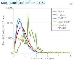
Fig. 4 presents the corrosion rate distributions used by each model with the corrosion rate derived from the repeated in-line inspections. The Markov model again best reproduces the empirical CR distribution. It not only provides the most accurate estimates for time evolution of the entire defect depth distribution, but also the best estimates for time evolution of defect sub-populations of different depths.
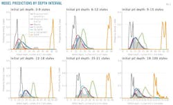
Fig. 5 confirms this, categorizing defects in the initial (1996-ILI) inspection into six-state depth intervals and plotting the depth distribution for each interval separately as a PDF with the depth distribution of the matched defects in the second inspection (2006-ILI). Fig. 5 presents these later depths in the form of a histogram, while also displaying the predicted distributions by the five models for each initial depth subpopulation.
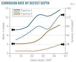
The results presented in Fig. 5 confirm the SVCR model and, to a lesser extent, the linear growth model as being incapable of reproducing the observed defect depths by the time of the second inspection. The SVCR model simply shifts the original distribution by a fixed amount to larger depth values without changing its shape. This result openly contradicts the stochastic nature of corrosion growth because the model cannot reproduce the inherent increase in the variance of the corrosion depth distribution over time (Fig. 6) (OGJ, Oct. 1, 2012, p. 122). Operators should therefore avoid using single-value corrosion rate distributions in reliability analyses, no matter what growth rate value is selected to create them.
The linear growth model, on the other hand, increasingly deviates from observed depth distributions for larger initial-depth values. The predicted distributions are also narrower than those experimentally observed. The linear growth model takes depth values from a certain part of the initial distribution and simply shifts them to larger depth regions, without considering the stochastic nature of the corrosion growth process. This behavior differs from what is detected experimentally. Fig. 5, for example, shows that narrow initial depth intervals (grey lines) evolve into wider distributions (grey histograms) covering a range of depth broader than the initial one.
The models that take into account soil properties (the GEVD-based and Markov models), by contrast, are capable of reproducing the experimental results. In most cases, the Markov model shows better performance than the GEVD-based models, which is quantitatively proven in Table 2, showing the quality index, Δmodel, for each one of the six cases presented in Fig. 5 is shown.
In all but one case (when initial defect depths were between 12 and 18 states), the Markov chain model has a quality index smaller than the TI-GEVD and TD-GEVD models. Fig. 5 and Table 2 show that the Markov model can account for not only the time dependence of the corrosion rate but also its dependence on defect depth (OGJ, July 20, 2009, p. 64; OGJ, July 27, 2009, p. 56).
The foregoing results lie in the ability of the Markov chain model to capture the influence of both depth and age of the corrosion defects on deterministic pit depth growth, together with its ability to reproduce the stochastic nature of the process, also as a function of the defect's depth and age. Comparing these capabilities with those shown by the rest of the models yields the following observations:
• The linear growth model uses only the uncertainty of the ILI tool to define the variance of the CR distribution to be associated with each defect. The estimated future pit depth distribution, therefore, strongly depends on the type of inspection tool used and not on the actual physical and chemical properties of the corrosion environment.
• The time-dependent and -independent GEVD models produce results close (yet inferior in quality) to those of the Markov chain model solely because the characteristics of the soil in which the example pipeline is corroding were known. The Markov remains, in the absence of such information, the only model that can fairly reproduce the time evolution of the corrosion defects from the depth data of the first ILI and the value of ν estimated using Equation 8 when repeated ILIs are available.
• The single-value CR model fails to reproduce the stochastic nature of corrosion and its dependence on the defect depths and ages, no matter what growth rate is used to construct it. As in the case of the linear growth model, its only advantage is ease of use.
The differences in the abilities of the different models correctly to describe the corrosion rate distributions and the corrosion growth process should markedly affect results of reliability estimations.
Reliability estimations
Researchers applied the described reliability framework to synthetic data; a hypothetical 100 km-long pipeline was used with OD D = 30 in. (762 mm), pwt = 0.45 in. (11.4 mm), and ultimate tensile strength UTS = 66,000 psi (455 MPa). These variables followed a normal distribution with standard deviation σD = 0.01 in (0.254 mm), σpwt = 0.045 in (1.14 mm), and σUTS = 3,000 psi (21 MPa), respectively. Assumed defects numbered 150 after 20 years in operation.
Calculations encompassed a time interval from 20 to 45 years (dt = 25 years), with a 2-year time step, and the soil-pipe parameters were taken as those found for the generic soil category. The chosen time range included the pipe lifetimes observed in the field survey carried out by the authors, in which the soil pit growth parameters were derived from the soil-pipe characteristics (OGJ, July 20, 2009, pp. 64-73). A total of 10,000 Monte Carlo simulations occurred.
Defect lengths pulled from a normal distribution had a mean mL = 0.45 in (11.4 mm) and standard deviation σL = 0.045 (1.14 mm). This length guaranteed rupture as the failure mode of all defects. The chosen lengths shouldn't alter the results of the reliability analyses, which have proven to have low sensitivity to uncertainties in defect length.4
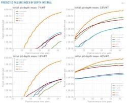
Investigating behavior of the different CR models as a function of defect depths used Log-normal distributions with different mean (μd) and variance (σ2d) values to model the pipeline's initial defect depth distribution. Fig. 7 shows a compendium of the results obtained for four different initial defect depth distributions with mean and standard deviation (all in mm) of (0.762, 2.540), (1.778, 3.810), (3.810, 5.080), and (4.572, 7.620). The mean depths correspond to 7, 16, 33, and 40% pwt, respectively.
The linear growth model underestimates the mean values of future depth for small depths (7 and 16% pwt), potentially leading to failure indices well below those predicted by the models that account for soil-pipe properties. The estimations made by the Markov model, meanwhile, are close to those of the TI- and TD-GEVD models, especially for long intervals (>15 years).
This coincidence is due to the corrosion parameters used in these models having been derived from a field survey, where the measured average defect depth was 2.02 mm (0.08 in) and the mean pipeline age was 23 years (OGJ, July 20, 2009, p. 64; OGJ, July 27, 2009, p. 56), making it logical to expect that the models work better for depths and times of this order.
For short time intervals, the Markov-chain-based model estimates failure indices slightly higher than those given by the GEVD models. The time-dependent GEVD model yields slightly higher failure indices than the TI-GEVD model.
For deeper defects (33 and 40% pwt), the linear growth and Markov models produce similar annual failure indices, although the former produces failure index values exceeding Markov results for deeper defects and longer exposure times. These indices are more than an order of magnitude higher than those estimated by the GEVD-based models, providing evidence that the latter models do not work well when the depth values or time intervals are far from those experimentally observed in the work where these GEV distributions were obtained (OGJ, July 20, 2009, p. 64). This example shows that the Markov model remains the best option when choosing CR distribution for pipeline reliability.
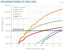
The next example involved application of the described reliability framework to the 1996-ILI data set. Fig. 8 shows the obtained failure indices for this experimental data set using the five analyzed corrosion rate distributions. In accordance with what was discussed earlier, the single-value CR and linear growth models overestimate the pipeline's failure index across the analyzed interval, leading to conservative predictions and shortened repair intervals.
A target reliability level of 10–3/km-year drawn in the form of a horizontal line in the failure index vs. time plot helps illustrate this observation. For this hypothetical target, the SVCR and linear growth models recommend maintenance actions 5 years before the Markov recommendation. As shown previously, the Markov prediction best describes the actual corrosion evolution (Fig. 3) and reliability results produced by this model can be considered closer to the pipeline's true reliability level.
The TI-GEVD and TD-GEVD models, on the other hand, underestimate the failure indices over the entire period and produce unrealistically long intervals before maintenance. For longer periods of time, however, the difference between the predictions made by these models and those of the Markov model become smaller, an observation consistent with the previously noted characteristic of the GEVD models as being suited only for corrosion data close to those previously found (OGJ, July 20, 2009, p. 64).3
With the passage of time, the defect depths become larger and uncertainty due to the stochastic nature of corrosion increases, as shown in Fig. 6, explaining why GEVD results approach Markov results over longer exposure times.
References
1. Leis, N., and Stephens, D.R., "An alternative approach to assess the integrity of corroded line pipe. Part I: Current status and Part II: Alternative criterion," International Offshore and Polar Engineering Conference, Honolulu, May 25-30, 1997.
2. Stephens, M., and Nessim, M., "A comprehensive approach to corrosion management based on structural reliability methods," International Pipeline Conference, Calgary, Sept. 25-29, 2006.
3. Caleyo, F., Velazquez, J.C., Valor, A., and Hallen, J.M., "Probability distribution of pitting corrosion depth and rate in underground pipelines: A Monte Carlo study," Corrosion Science, Vol. 51, Issue 9, pp. 1,925-34, September 2009.
4. Caleyo, F., Gonzalez, J.L., and Hallen, J.M., "A Study on the Reliability Assessment Methodology for Pipelines with Active Corrosion Defects," International Journal of Pressure Vessels and Piping, Vol. 79, Issue 1, pp. 77-86, January 2002.
