LOUISIANA HAYNESVILLE SHALE—2: Economic operating envelopes characterized for Haynesville shale

Mark J. Kaiser
Yunke Yu
Louisiana State University
Baton Rouge
The Haynesville shale has grown into the largest gas shale play in the US due to favorable geologic conditions and technological improvements in drilling horizontal wells and stimulation treatment. Unconventional gas resources are abundant, but their development is particularly sensitive to technologic risk, geologic uncertainty, and gas price.
Misunderstanding aboveground risk, however, can have an unpleasant effect on project economics.
The two defining characteristics of shale gas development in Louisiana's Haynesville shale are the high costs of drilling and completion and the high degree of uncertainty surrounding physical and economic parameters that affect project returns. Project risk is caused by uncertainty from unforeseen or unknowable conditions or events that affect costs or performance.
The purpose of this article, the second of three parts, is to examine the price sensitivity of Haynesville wells. We characterize the operating envelope under which Haynesville wells are economic and describe the profit space based on a technical review of cost characteristics. Two-variable factor models are combined with type curves to construct before and after-tax profit matrices.
The majority of Haynesville wells fail to break even on a full-cycle basis at prevailing gas prices. This harsh economic reality will control future activity after new entrants fulfill their drilling requirements.
For $6/Mcf gas, average wells are expected to generate pretax returns between 1% and 11.5% for $1 to $0.50/Mcf operating expenses and $7.5 million capital expenditure. P10 wells are expected to generate a pretax return of 52% for $7.5 million to 25% for $10 million capital expenditures and posttax returns of 20% to 40%. We show that gas prices during the first year of production are an important determinant in profitability.
Shale play economics
For shale gas wells to be profitable, they must produce at sufficient rates and volumes to recover the high cost of drilling and completion. The tradeoff between perforated length, completion strategy, and production is a key consideration in cost and returns. Shale wells produce smaller volumes per well compared with conventional resources, and typically, per-well profit margins are smaller. Recovery factors are also much lower than in conventional gas plays, typically on the order of 20-30%.
Unconventional reservoir systems are governed by a large number of factors and interrelationships that are difficult to accurately discriminate. Geologic and reservoir engineering and economic modeling have lagged the science of hydraulic fracturing, but progress continues to be made.
Production risk is higher in shale plays because of the need to use advanced technologies and constraints imposed by the reservoir. Completion technology and geologic controls are considered the primary determinant of production and economic success. Completion strategies involve many factors, including lateral length and number of stages, method of isolation, completion and fracturing techniques, and proppant type and concentration. Strategies evolve with experience and experimentation, and performance are influenced by many interrelated parameters.
Cost data
Acquisition
Over the past 3 years, lease bonuses on state lands in the Haynesville region have ranged between $5,000 and $25,000/acre and averaged $9,000/acre. The average royalty rate on state land has ranged from 22.5% to 28.5%, while royalty interest and overrides on private land generally range from 20% to 30%.
Drilling and completion
Drilling and completion is the main cost in shale gas plays. In 2009, the average onshore horizontal gas well in the US was drilled an average of 10,025 ft at a cost of $8.6 million, or $842/ft, according to the American Petroleum Institute. The average Haynesville well has a measured depth of 16,654 ft and would have been expected to cost $14 million in 2009.
In the third quarter of 2008, Chesapeake Energy Corp. reported that the drilling and completion cost of a Haynesville well averaged $9.5 million and required 64 days from spud to rig release. By the second quarter of 2009, well construction cost $7.9 million and required 47 days to rig release.
In 2010, Encana spent $1.261 billion and drilled 106 wells in the Haynesville for an average $11.9 million/well. In 2009 and 2008, Encana reported spending $541 million and $137 million and drilling 49 and 7 wells, or $11 million/well and $19.6 million/well, respectively.
Lease operating expenses
Lease operating expenses (LOE) are those costs associated with work physically performed at the work site or specifically and exclusively for operations.
Operating costs vary between leases and with the inventory of producing wells and change with commodity prices (because of changes in lease fuel and production taxes); age (chemical treatment and monitoring, corrosion, and scale); the number and type of wells and surface facilities; product stream (gas, oil/gas) and volume; water production and disposal options; and well servicing requirements (workovers).
EXCO Resources reported Haynesville shale LOE for 2010, 2009, and 2008 as $0.50/Mcf, $0.80/Mcf, and $0.85/Mcf; workover expenses are reported as $0.11/Mcf, $0.12/Mcf, and $0.14/Mcf. Chesapeake reported Haynesville/Bossier shale production expenses and ad valorem tax expenses for 2010, 2009, and 2008 to be $0.27/Mcf, $0.39/Mcf and $1.33/Mcf, respectively.
General and administrative
General and administrative (G&A) expenses covers payroll, media relations, stock-based compensation, and associated costs excluding cost capitalized to properties. Company size, property distribution, and number of administrative staff and compensation impact G&A expenses.
Chesapeake reported G&A expenses as $0.45/Mcf, $0.38/Mcf, and $0.45/Mcf for 2010, 2009, and 2008, respectively.
Model assumptions
Shale plays are exposed to the same price uncertainty impacting conventional production, but because of high initial production rates and steep decline, exposure is concentrated across a much smaller time window which amplifies the potential investment risk.
The price received for natural gas is largely a function of regional supply and demand conditions which is impacted by general economic conditions, storage volumes, weather, and other seasonal conditions, including hurricanes and tropical storms. Gas prices are assumed to be flat over the life cycle of production and range between $4 and $10/Mcf.
Royalty is levied on gross production at a rate of 20-30%. Well-spacing requirements are assumed to range from 80 to 640 acres/well. Production is assumed gas with no commercial liquids.
In 2010, most wells in the Haynesville were drilled and completed for $7 million-$10 million. We assume capital expenditures range between $5 million and $15 million and include the cost to tie in to existing infrastructure.
LOE is assumed to range between $0.25 to $2/Mcf. We assume no additional capital expenditures (e.g., restimulation) are required through the production life cycle. Unit cost of production increases over time because of the need for compression, maintenance related to corrosion, equipment repairs, water treatment and disposal, etc., but we consider LOE constant and do not inflate. G&A expenses are not considered.
Gas wells that produce more than an average monthly rate of 250 Mcfd are charged a severance tax that is adjusted annually. Severance tax rates are correlated with gas price and vary approximately linearly from $0.18/Mcf for $4/Mcf gas to $0.45/Mcf for $10/Mcf gas.
A horizontal well severance tax exemption applies to any well or any horizontal recompletion where production commenced after July 31, 1994. All severance tax on a horizontal well is suspended for a period of 24 months or until payout of drilling and completion cost is achieved, whichever comes first.
Property tax is assessed on surface and subsurface equipment according to depth brackets based on the uppermost producing interval of the well. Millage rates usually vary from $75 to $150 per $1,000 of assessed value. Property tax is not considered.
All capital expenditures occur in the year of first production, and we apply midyear discounting using a discount rate that ranges from 8% to 20%.
The percentage of intangible (expensed) to tangible (capitalized) cost is unknown and assumed to range from 40% to 60%. There are many lives of equipment, ranging from 3 to 25 years, and either 150% or 200% declining balance may be used depending on the life of the asset. We have used 150% declining balance over a 5-year time period as an average.
Wells are abandoned at the economic limit of 90 Mcfd or when the reservoir pressure declines to the point where the cost of compression is no longer economical. Abandonment cost is not considered.
Analysis is performed before and after federal income tax. Federal income tax is levied on gross revenue less royalty, operating costs, dry hole costs, intangible development costs, depreciation of other exploration costs, and tangible development expenditures. We do not consider depreciation of leasehold acquisition costs or G&G expenses. Losses may be carried forward for a maximum of 10 years. Federal tax rate is assumed to range from 35% to 50%.
Two-factor model
Discounted before and after cash flow analysis is performed on average production profiles for 6-24 month vintage Haynesville wells (Fig. 1) for the range of input parameters summarized in Table 1.
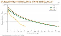
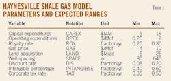
P50 is the base (average) case and P10 (optimistic) and P90 (pessimistic) represent the expected bounds for the range of well performance. The input variables include capital expenditures (CAPEX), operating expenditures (OPEX), royalty rate (ROY), acreage cost (LAND), land spacing (SPACE), discount rate (DIS), intangible percentage of drilling and completion cost (INTANGIBLE), and corporate tax rate (TAX). The output variables are NPV and IRR.
P10 curves obviously yield the most favorable economics and P90 the least favorable, and the scale of these differences provide an indication of the range of results and the potential investment risk.
Also, before-tax analysis will yield more favorable results relative to an after-tax assessment and both are presented for comparison.
Tax on income is difficult to evaluate without detailed information and is usually considered to have a modest impact on development decisions. The nature of tax assessment is uncertain and our ability to capture subtle aspects is limited.
Model results
Gas price, capital expenditure
In Table 2, we vary gas price and capital expenditures and compute NPV fixing all other model parameters at their expected value, specifically, royalty rate at 25%, $9,000/acre lease cost, 80-acre well spacing, $1/Mcf operating expenses, 10% discount rate, 50% tangible expenditures, and 35% tax rate.
At $4/Mcf gas price, no value is created under most CAPEX scenarios except for P10 wells that can be brought in for less than $7.5 million. In the after-tax case, the $5 million well will create marginal value. To hold acreage in low price environments, operators target high quality shale prospects, but if the well comes in at average rate, it is unlikely to be economic.
At $6/Mcf gas price, P10 wells are profitable through capital expenditures of $12.5 million before-tax and $7.5 million after-tax. For P50 wells, the profit window shrinks and no value is created unless CAPEX is held under $10 million (before-tax) or $5 million (after-tax). As long as producers can maintain cost controls, the average well is likely to be profitable at $6/Mcf, and thus, $6/Mcf gas will stimulate activity and investment in the region.
In Fig. 2, the NPV range for P50 wells as a function of capital expenditures for gas prices between $4 and $10/Mcf is shown. At $8/Mcf gas and higher, P10 wells are profitable for most of the capital expenditure scenarios depicted, while for the P50 well present value is positive through $12.5 million (before-tax) and $10 million (after-tax).
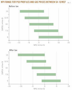
P90 wells will not make any money under any of the scenarios depicted except the unlikely combination of $10/Mcf gas price and $5 million CAPEX. P90 wells will not return their investors capital.
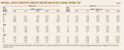
Capital expenditure, operating expenditure
In Table 3, capital and operating expenditures are varied assuming a $5/Mcf gas price, 25% royalty rate, $9,000/ac lease cost, 80-acre well spacing, 10% discount rate, 50% tangible expenditures percentage, and 35% tax rate.
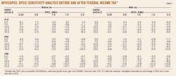
In the P10 stairs in the before-tax matrix, OPEX increases by $0.25/Mcf in the first horizontal increment, while CAPEX is reduced each vertical step by $2.5 million. Each step up expands the profit window because the reduction in upfront investment dominates the impact of the increase in OPEX over the life of the well.
According to the before-tax assessment, value is created when OPEX ≤ $1/Mcf and CAPEX ≤ $10 million, or when OPEX = $0.25/Mcf and CAPEX ≤ $12.5 million. Haynesville wells cannot be drilled and completed for less than about $7 million, so $5 million wells are not currently realistic. For P50 wells, the profit window shrinks considerably with value created only when CAPEX ≤ $7.5 million and OPEX ≤ $0.5/Mcf. All profit windows shrink when taxes are included.
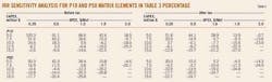
Rate of return
Pre- and posttax IRRs for the P10 and P50 wells depicted in Tables 2 and 3 are summarized in Tables 4 and 5. The signs and profit windows indicate a broad range of returns.
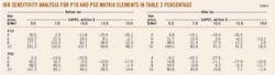
For $6/Mcf gas, average wells are expected to generate pretax returns between 1% and 11.5% for $1 to $0.50/Mcf OPEX and $7.5 million CAPEX. P10 wells are expected to generate a pretax return of 52-25% for $7.5 million to $10 million CAPEX and posttax returns of 20-40%. For $6/Mcf gas, average wells will generate a pretax return between 7.6% to 33% for $10 million to $7 million CAPEX and $0.50/Mcf OPEX.
Impact of first year prices
One of the most important factors in the success of a shale gas drilling program is the commodity price during the first year of production and, for Haynesville wells, the first several months after a well is brought on line is an important determinant in profitability.
This is not entirely unexpected, of course, and follows from the high initial production rates and steep decline curves characteristic of the play.
Although operators can shut in production in low price environments, invested capital requires a return and there are limitations on the ability to match output with high commodity prices.
We assess the impact of first year prices on profitability. In Table 6, we assume the first year gas price is $7/Mcf followed by the prices depicted in column one for the second year forward. All other model assumptions are the same as in Table 2 for the before-tax P50 analysis.
The profit envelope expands significantly and NPV is greater for entries when gas prices are less than $7/Mcf. If first year gas price is $7/Mcf, even $4/Mcf future gas is economic for capital expenditures less than $7.5 million. When future gas prices are less than $7/Mcf project value will increase. If future gas prices are greater than $7/Mcf, however, project value will decrease because the first year price reduces the value of the well. For example, for $8/Mcf gas and $10 million CAPEX, Table 6 yields NPV = $2.0 million while Table 2 yields NPV = $3.3 million.
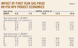
The difference in the individual components of Table 6 and Table 2 reflects the added value high first year prices provide. For $6/Mcf gas (year ≥2) and $7.5 million CAPEX, Table 6 yields a project value of $3.0 million, while Table 2 yields $1.6 million, a difference of $1.4 million due to the first year price differential.
If first year prices plummet to $3/Mcf when first production is achieved, the results are disastrous. The profit envelope shrinks significantly and even $10/Mcf future gas price will only recover marginal returns.
NEXT: The operating envelope under which Haynesville shale wells are profitable are expressed in functional form.
More Oil & Gas Journal Current Issue Articles
More Oil & Gas Journal Archives Issue Articles
View Oil and Gas Articles on PennEnergy.com