World peak oil production still years away

Brian Towler
University of Wyoming
Laramie, Wyo.
Peak world oil production rate depends on economics and is unlikely to occur before 2018, and rising oil prices and technological developments may further delay this peak.
When production rate eventually does peak, however, the decline side of the curve will not mirror the growth side as predicted by Hubbert.1 2
Oil has been the number one energy source in the world since the middle of the 20th century. But ever increasing demand has caused its price to spike in recent years and only world economic crises have tempered demand and brought down its price,
Demand and price, however, likely will increase again when the economy recovers. The world still has much oil, and production will continue to meet demand for some time.
Peak oil theory
Peak oil theory grew out of a 1956 paper1 by Marion King Hubbert who was a geologist-geophysicist at Shell Research Lab in Houston.
The theory holds that world oil supply has peaked already or likely will peak soon, thus putting an upward pressure on oil price.
In his 1956 paper, Hubbert proposed that any finite resource, such as oil, gas, coal, or uranium, follows a bell-shaped production curve. At some point, production reaches a peak and begins to decline, and the decline will mirror the rise in production.
The peak production rate and the timing of the peak depend on the total reserves that exist and are discovered in the future. Because the two sides of the bell-shaped curve mirror each other, production will start to decline after half of the world's reserves are produced.
Hubbert's theories have garnered much credibility after he successfully predicted the rise and fall in US oil production. His prediction, however, of world oil production rate peaking in 2000 and falling rapidly after 2000 has not proven true. Eleven years later, world oil production rate continues to rise in accordance with world demand.
His theories still have much support and many expect oil production to peak soon and then fall rapidly. They then expect the world to be starved of energy with resource wars to follow in a struggle for controlling rapidly depleting remaining resources.
Oil is a finite resource and eventually world oil production will peak in the distant future and then run out. But in this article, I will show that the world still has plenty of resources and when production eventually does peak, it will decline less rapidly than Hubbert predicted.
Probably the leading exponent of Hubbert's theories is Ken Deffeyes, a geologist who worked at the Shell Research Lab in the early 1960s as a colleague and protege of Hubbert. Deffeyes published three books that espouse his theories.3-5
His first book in 2001 forecast an imminent start of an oil shortage and dire consequences for the world economy. He forecast that oil production would peak in August 2004.
His second book in 2005 slightly revised the forecast for the world oil production peak to late 2005, and in the preface to the paperback edition (written in 2006), he wrote that Dec, 16, 2005, was the actual date that world oil production peaked. In the preface of the book's 2008 edition, he triumphantly says, "I told you so."
In his third book in 2010, he ignores the fact that world oil production was still rising and continues to insist that production peaked in 2005, and points to the rapid increase in the oil price during the last 6 years.
Hubbert's model
For his forecasts, Hubbert asked Wallace Pratt and Lewis Weeks, both from ExxonMobil subsidiaries, to provide estimates of the ultimate recovery of oil and gas in the world and US.
But determining the ultimate reserves to be discovered and produced in the future was somewhat of a guessing game that Hubbert was not comfortable with. He then realized that with the right model, he did not need to guess. The production data itself could be fitted to the model to determine ultimate reserves.
From this model, he developed some mathematical methods for forecasting ultimate reserves. These methods depend on his assumed model for production, and the exact equations for the bell-shapped curve. This technique removed some uncertainty about ultimate reserves.
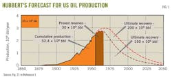
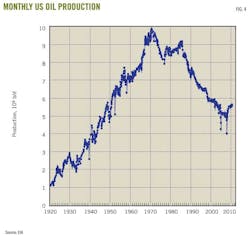
Three of Hubbert's bell-shaped curves show his forecast for oil production in the US (Figs. 1-3).1 He used two estimates from Pratt and Weeks for ultimate oil reserves of 150 billion and 200 billion bbl. With the higher estimate, he forecast that US oil production would peak in 1970 at 3 billion/year (8.2 million b/d).
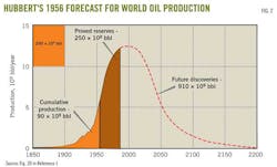
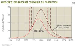
Fig. 3 shows that actual US oil rate peaked in November 1970 at 10 million b/d). In 1970, the US actually produced 3.5 billion bbl.
Hubbert's prediction was remarkably successful and this has given much credence to his method that came to be known as peak oil theory or Hubbert's peak.
The plot in Fig. 2 does have two deviations. After the November 1970 peak, US oil production declined for 6 years in the manner predicted by Hubbert. But from January 1977 to February 1986, oil production rose again forming a secondary peak at 9.14 million b/d.
This deviation and secondary peak was due to oil production from Prudhoe Bay and Kuparuk fields on Alaska's north slope. Hubbert might argue that he did not take this area into consideration and that, excluding the Alaska oil production, the US oil production from 1970 did decline in the manner predicted.
The other deviation is the incline since 2008 that was caused by the ramping up of oil production from the deepwater Gulf of Mexico and from the unconventional Bakken oil play in North Dakota.
These oil sources, if allowed to continue, likely will cause US oil production to keep increasing to form a tertiary peak sometime after 2020. Once again, Hubbert might argue that he was talking about conventional onshore oil and did not consider these unconventional plays.
Despite these two deviations, Hubbert's predictions for US oil production were remarkably accurate.
Hubbert also forecast world oil production (Fig. 3), based on ultimate oil reserves of 1.25 trillion bbl. His forecast peaked at 12.5 billion bbl/year (34.25 million b/d) in 2000. Later in his 1969 paper, he revised his estimate with two ultimate recoveries of 1.35 trillion bbl and 2.1 trillion bbl.2 The more optimistic 2.1 trillion bbl estimate again peaked in 2000 at 37.5 billion bbl/year (103 million b/d).
Hubbert's forecasts obviously depend on knowing how much oil can be discovered and produced, and critics of his method say that this number is only a guess. Can we really know how much oil is going to be eventually discovered and produced in the world?
Supporters point out that the timing of the peak is not sensitive to the actual assumed ultimate recovery. Indeed, from Figs. 3 and 5 three ultimate recoveries, ranging from 1.25 trillion to 2.1 trillion bbl, have a peak around 2000. Hubbert tackled this problem and, borrowing from the mathematics of biological population growth and decay, he devised a mathematical method for forecasting ultimate recovery, designated here as Qmax.
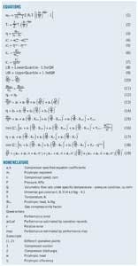
The equations he used start with Equation 1 in the equation box for the cumulative production Qt at time t. The production rate Qt at time t is the derivative of Qt with respect to t (Equation 2). Equation 2 is the basis for the production plots in Figs. 1-4.
If this model is correct for the production data then, as long as we have early time data, we can fit the data to the model and determine the ultimate recovery Qmax, as well as the parameters a and b.
Several methods will determine the parameters from the data. Hubbert recommended the combining of Equations 1 and 2 to give Equation 3. Equation 3 when rearranged gives Equation 4.
Equation 4 says in a plot of qt/Qt vs. Qt, parameter b is the intercept on the y axis and ultimate recoverable oil Qmax is the intercept on the x axis. This plot can be drawn at any time, even before the peak rate.
Taking the derivative of Equation 2 and setting it equal to zero finds the timing of the peak (Equation 5).
Equation 5 requires parameter a, which was not determined from the plot of Equation 4. The easiest way to determine parameter a is to rearrange Equation 1 as Equation 6.
Equation 6 says the slope of (Qmax/Qt)–1 vs. e–bt equals a. This second plot assumes that b and Qmax were determined from a plot of Equation 4.
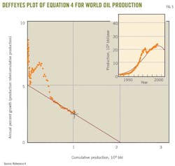
Deffeyes plotted Equation 4, using world production data until 2005 (Fig. 5). His extrapolation to the x axis shows a Qmax of 2 trillion bbl. Note that, before 1983, the data were increasing and deceasing and had not formed a straight line. But from 1983 to 2005, the data lie on a straight line as Hubbert's theory predicts.
Deffeyes also estimated the time of the peak rate directly from his plot because if the ultimate recovery is 2 trillion bbl then the peak oil rate will occur when cumulative production is 1 trillion bbl. This occurred in 2005 and led Deffeyes to predict 2005 as the year of peak production.
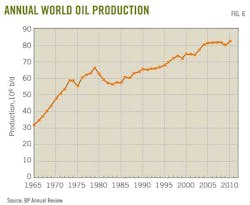
But world oil production did not peak in 2000 or in 2005. Fig 6 shows annual world oil production still was increasing in 2005
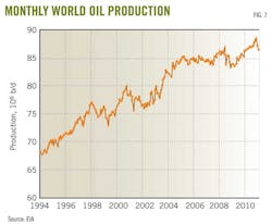
Fig. 7 shows the world's monthly oil production. Although production occasionally declines, the overall trend on both Figs. 6 and 7 is up and shows no evidence of a peak.
The occasional dips in production during the past 45 years are due to demand decreases rather than supply decreases. This, however, does not stop pundits from declaring that world oil production has peaked every time production decreases from 1 year to the next or even from 1 month to the next.
Data for Fig 6 are from the BP Annual Statistical Review, while the data for Fig. 7 are from the US Energy Information Agency (EIA). Any discrepancies between the two plots are due to the two different data sources. What is important is that both plots show a consistent upward trend in world oil production.
Production did have a secondary peak in 1979 and declined 1979-83. This was caused by a steep increase in world oil price that resulted in decreased demand as people reduced their use of transportation fuels.
But from 1983 to the present, oil demand has increased steadily and been matched by supply.
The world economic crisis in mid 2008 tempered demand and caused a production decline in late 2008. But from January 2009 to January 2011, production again rose.
The uprisings in Libya and other Middle East countries in early 2011 have caused a new round of price increases and subsequent decrease in demand for oil, but this too is expected to be temporary.
So what is wrong with the Hubbert model and the analysis of his supporters that has caused their forecasts about the timing of peak oil to be off? I believe that the Hubbert model essentially is correct under a constant price and constant technology scenario. When the oil price increases, however, the value of Qmax also increases as more oil becomes economic to produce. Technology also has an effect.
Technological breakthroughs bring more oil reserves into production even under a constant price scenario. Additionally, an increasing oil price is an incentive for developing new technologies that also increase oil supply. Price increases and technological breakthroughs seem to unlock large volumes of oil that previously were uneconomic to produce.
In the past 20 years, large reserves in the Canadian oil sands in Alberta have come on stream. New fracture stimulation and horizontal drilling technologies also have unlocked large reserves of tight oil, tight gas, and shale gas.
Alberta's oil sands currently have 170 billion bbl of booked reserves and possible reserves may be as high as 1 trillion bbl. In comparison, slightly more than 1 trillion bbl have been produced in the world and Deffeyes and Hubbert estimated that 1 trillion bbl of conventional oil remains to be produced.
Horizontal wells and multizone fracture stimulations are unlocking hundreds of billions of barrels from the Bakken formation in North Dakota, Montana, Manitoba, and Saskatchewan. The success in the Bakken also is opening up more formations to successful production, such as the Eagle Ford in Texas, Granite Wash in Oklahoma and the Texas Panhandle, Niobrara in Colorado and Wyoming, Monterey in California, and Utica in eastern Ohio.
Vast quantities of oil also have been discovered in deepwater Gulf of Mexico and Santos basin off Brazil.
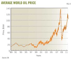
As these technologies mature they will find applications in many other areas in the world. The price increases of 2007-08 and 2011(Fig. 8) have accelerated deployment of these new technologies as well as economic development of other marginal reserves.
From 1986 to 2005, oil prices remained relatively constant at about $20/bbl, but warnings from peak oil theorists may have caused the market to start anticipating supply shortages and this and the political upheavals in the Middle East in 2011 have driven up oil prices.
At the same time, increased oil prices have led to an increased value of the world's remaining oil reserves and delayed the year for peak production. These developments not only affect Qmax and tpeak but will also affect the production decline on the back side of the Hubbert curve.
The history of US gas production has considerable relevance to world oil supply trends. Based on US gas production, the sliding down on the back side of the curve as in Hubbert's forecasts or that theorists expect will not occur.
At this point you might also ask why did the Hubbert model work so well in the prediction of the US oil supply but does not seem to be working, and will not continue to work, for predicting the world oil supply. The answer is simple. The oil market is a world market and the US oil production peaked and declined amidst a relatively constant world oil prices.
Even though US supply was decreasing, world supply was stable and prices remained relatively constant from 1986 to 2005. The Hubbert model works as long as the price remains stable. But the world price is now ramping upwards, and this will change profoundly the dynamics of the Hubbert model.
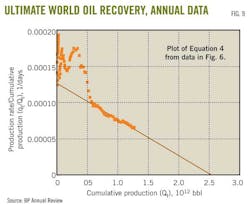
For example, Fig. 9 is a plot using Equation 4 of annual production data from Fig. 6. Extrapolating the data to the x-axis gives a Qmax of 2.54 trillion bbl. This compares with the 2 trillion bbl that Deffeyes got using this same data to 2005.
Between 2004 and 2010, oil price increased to $100/bbl from $20/bbl, and it became economic to develop the tight oil in the Bakken and Eagle Ford formations, the heavy oil sands in Canada, and the deepwater oil in the Gulf of Mexico and Santos basin. In fact, another half trillion bbl became economic to produce.
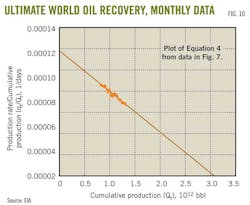
The monthly data (Fig. 7) in a similar plot extrapolate to 3.055 trillion bbl. Of this, 1.3 trillion bbl has been produced, leaving about 1.7 trillion bbl still to be found and produced.
EIA currently lists world oil proved reserves as 1.3 trillion bbl, meaning that only 400 billion bbl remain to be found.
These estimates are a function of oil price and likely conservative. But since this data are probably the most reliable available data, this estimate is probably the most reliable estimate under current economics.
It seems that more oil appears all the time. This is because of economics. If and when oil prices increase again and stay up, these values will increase again.
The exponential coefficient parameter a is from a plot of Equation 6. With this plot and monthly data from EIA, the value of a is 162.66. The y-axis intercept in Fig. 10 provides a value for b of 0.00011733 days–1.
Using these values of a and b in Equation 5 results in the peak rate occurring in 43,396 days from an arbitrary time zero, which in this case was Jan. 1, 1990. Oct. 23, 2018, is 43,396 days from time zero.
I am not saying that the world oil production will peak in October 2018 but that using Hubbert's model and EIA's monthly world oil production data results in a peak rate on Oct. 23, 2018.
If oil prices remain constant for the next 7 years and without major technological breakthroughs, this date may prove to be about accurate. But I do not expect that this will be the case and this date will probably move again.
US gas supply
US gas supply trends have much relevance to world oil supply behavior. In his 1956 paper1 Hubbert forecast US natural gas production (Fig. 11) peaking around 1972 at about 14 tcf/year (38 bcfd) with a Qmax of 850 tcf.
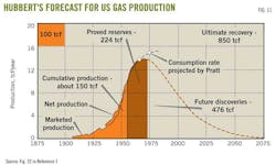
His figure also showed projected gas consumption rate that continued to increase after gas production peaked. Pratt supplied this projection.
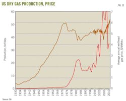
Fig. 12 shows that actual US dry gas production had a peak in 1973 almost the same as Hubbert forecast but at a higher peak rate of 60 bcfd.
Gas consumption continued to increase after the peak as his plot showed and the shortfall that occurred after 1973 was met by imports, mostly by pipeline from Canada.
Fig. 12 shows annual gas production until 1997 and monthly production after 1997. The decline in production after the 1973 peak, however, did not happen according to Hubbert's forecast. The rate began to decline for 2 years and then remained constant for 5 years. The decline then resumed, finally bottoming out at 44 bcfd in 1986.
Since then, production has increased steadily and more sharply in 2006. Production today is about 63 bcfd of dry gas, or more than the 1973 peak.
If the production decline had mirrored the front side of the peak, in 2010 we would expect a gas production of about 6 bcfd, the same as in 1936.
The Hubbert method failed to forecast what has happened on the back side of the US gas production curve. The reason is economics. Once US gas supply peaked and a gas shortage developed, the gas price began to increase. The increased price shook loose gas that previously was uneconomic to produce and the industry began to develop technologies to find and produce coalbed methane, tight gas, and shale gas. This unconventional gas now accounts for the majority of current US gas supply.
The US surpassed Hubbert's estimate of the total ultimate recovery of 850 tcf in 1997 and so far has produced more than 1,120 tcf without reaching a new peak.
Fig. 12 also illustrates the effect of price on supply. The steep run up in the gas price after the peak created new supplies, causing the Hubbert model to fail on the back side.
The same thing did not happen for US oil supply because the oil market is a global market. The price of US oil could not be pushed up in the same way that gas price was pushed up because the US always has imported a large portion of its oil. US oil producers were constrained by world oil price, which remained relatively low until recently.
In contrast, apart from Canadian supplies and a small and expensive LNG market, the US gas market is relatively insular.
This analogy between oil and gas illustrates that economics affect the supply of commodities such as oil and gas. In the case of world oil supply, the oil price has increased recently before reaching peak oil production. This in turn has delayed the peak and increased total cumulative production.
When world oil production eventually does peak, as it must, the back side of the curve will not mirror the front side as Hubbert had forecast. It probably will not look like the back side of the US gas supply curve either. Economics and technology will control the curve, which at this time is difficult to predict.
In his 2010 book,5 Deffeyes presents several proofs and analogies to show that the production curves must be symmetrical and that its back side must mirror its front side. All these proofs depend on a constant oil price, which clearly will not happen.
If and when oil production does peak, the shortage of supply will push oil price up and the back side will not mirror the front side. The fact that the US gas production curve is asymmetrical is an indication of the fallacy of Hubbert's assumption and the subsequent proofs by Deffeyes
One scenario in which the back side of the curve might mirror the front side is if $100/bbl gas-to-liquids and coal-to-liquids technologies becomes economic. If the world shifted rapidly to these technologies and supply were maintained at a high enough rate to keep oil price constant, then the back side of the production curve might mirror the front side.
World oil reserves
Table 1 lists the 20 countries with the most proved oil reserves. This includes heavy oil sand reserves, which are the majority of reserves in Venezuela and Canada.
Reported world proved oil reserves are 1.3 trillion bbl, although some peak oil theorists believe that this value is incorrect. They believe that some OPEC members inflate their reserves so that they can receive a higher production allocation. I have no reason to believe that these numbers are not approximately accurate and reasonable.
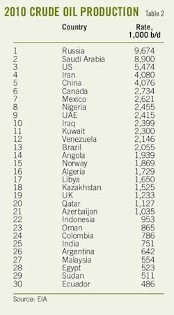
Table 2 lists the world's top 30 producing countries. Their production rates should approximately correlate to reserves. More reserves should have a higher production rate.
In this respect, the US does not follow this correlation. It is producing 5.47 million b/d from only 20 billion bbl of reserves. Countries such as Canada and Venezuela have the capacity to increase production, although most of their reserves are very heavy oil, which limits production rates because of the low oil viscosity.
If Saudi Arabia has 263 billion bbl of reserves, and I believe that it does, it could also increase production substantially as it has done at times. Saudi Arabia has elected to operate as the world's swing producer, increasing its production when the world demand rose and decreasing production when demand lessened.
Saudi Arabia would increase production happily if the world demanded it, and it is aware that a too high oil price decreases demand and starts the world to look for alternatives.
The US produces oil at about half the rate of Saudi Arabia with less than one tenth of the reserves.
Other countries also have capacity to increase their production, and one way to gauge this is to calculate reserves life at current production rates.
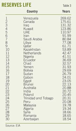
Table 3 lists the 30 countries with the most reserves life. Note that the top two countries are Venezuela and Canada because of their heavy oil reserves. Any country with more than 30 years of reserves life probably has the potential to increase its production.
The US does not appear on this list because US reserves life is only 10.35 years. The country cannot keep producing oil at its current high rates relative to its reserves unless continual drilling of new wells develops more resources. Its production rate will plummet if drilling stops.
References
1. Hubbert, M.K., "Nuclear Energy and the Fossil Fuels," API Drilling and Production Practices, Spring Meeting, San Antonio, Mar. 7-9, 1956.
2. Hubbert, M.K., "Energy Resources", in National Research Council Committee on Resources and Man, W.H. Freeman, San Francisco, 1969.
3. Deffeyes, K.S., Hubbert's Peak, The Impending World Oil Shortage, Princeton, NJ: Princeton University Press, 2001.
4. Deffeyes, K.S., Beyond Oil, The View from Hubbert's Peak, New York: Hill and Wang, 2005.
5. Deffeyes, K.S., When Oil Peaked, New York: Hill and Wang, 2010.
The author

More Oil & Gas Journal Current Issue Articles
More Oil & Gas Journal Archives Issue Articles
View Oil and Gas Articles on PennEnergy.com